The documentation for OpenCV is described as some of the best I’ve ever seen, but what really exists are hundreds of (good) unanswered questions on their forums (e.g.), a reference that’s about like reading source code, seriously uncommented source code examples, and tutorials that don’t actually exist yet.
However, the sample programs are functional and quite illustrative. It is probably best to start with them and find the demo that is closest to what you need and then copy its major components.
References
-
Tutorials
-
Joeseph Redmon teaches a computer vision class.
Acquiring OpenCV Source
Normal Debian people doing the normal thing.
sudo apt install libopencv-dev python-opencv opencv-docNote that opencv-doc includes the Python examples
(/usr/share/doc/opencv-doc).
In Debian 10 this seems to have worked for me for Python modules.
sudo apt install python3-opencv python3-numpyNow it is possible to import cv2 which is good.
From Source
OpenCV now uses GitHub.
git clone https://github.com/opencv/opencv.gitFormerly they used CVS.
cvs -d:pserver:anonymous@opencvlibrary.cvs.sourceforge.net:/cvsroot/opencvlibrary login
cvs -z3 -d:pserver:anonymous@opencvlibrary.cvs.sourceforge.net:/cvsroot/opencvlibrary co -P opencv
Change to the opencv source directory you just acquired and do the
cmake dance.
$ mkdir build
$ cd build
$ cmake ..
$ make
I had trouble with the Eigen library not being found. I had to make a symlink like so.
cd /usr/include
ln -s eigen3/Eigen
I also had heroic struggles getting FFMPEG to be detected and incorporated properly. This is what that problem looks like.
--   Video I/O:
--     DC1394:                      YES (2.2.5)
--     FFMPEG:                      NO
--       avcodec:                   YES (57.64.101)
--       avformat:                  YES (57.56.101)
--       avutil:                    YES (55.34.101)
--       swscale:                   YES (4.2.100)
--       avresample:                YES (3.1.0)
--     GStreamer:                   NO
--     v4l/v4l2:                    YES (linux/videodev2.h)
This bug report is very much on target however, none of the "solutions" worked for me so far.
Maybe this approach will work: https://mindchasers.com/dev/ubuntu-opencv
Structural Overview
- CXCORE
-
Basic structures and algorithms, XML, drawing functions
- CV
-
Image processing and vision algorithms
- MLL
-
Machine learning, statistical classifiers, clustering
- HighGUI
-
GUI, image and video IO
- CvAux
-
Misc extensions and fancy functionality that is not well documented.
Acronyms
- IPL
-
Note also that many structures and types are named things like
IplImage. This cryptic name refers to the Intel Image Processing Library. - ROI
-
Region of Interest, not return on investment.
- COI
-
Channel of Interest
Modules
-
core
-
#include "opencv2/core/core_c.h"- Old C version. -
#include "opencv2/core/core.hpp"- New C++ version.
-
-
imgproc
-
#include "opencv2/imgproc/imgproc_c.h"- Old C version. -
#include "opencv2/imgproc/imgproc.hpp"- Newer C++ version.
-
-
highgui
-
#include "opencv2/highgui/highgui_c.h"- Old C version. -
#include "opencv2/highgui/highgui.hpp"- Newer C++ version.
-
-
calib3d - Calibration.
-
#include "opencv2/calib3d/calib3d.hpp"
-
-
features2d - Feature tracking.
-
#include "opencv2/features2d/features2d.hpp"
-
-
objdetect - HOG,SVM
-
#include "opencv2/objdetect/objdetect.hpp"
-
-
ml
-
#include "opencv2/ml/ml.hpp"
-
-
flann - fas library approximate nearest neighbors
-
#include "opencv2/flann/miniflann.hpp"
-
-
video - tracking, segmentation
-
#include "opencv2/video/video.hpp"
-
-
photo - new module for computational photography.
-
#include "opencv2/video/photo.hpp"
-
-
contrib - Possibly non-free.
-
#include "opencv2/contrib/contrib.hpp"
-
-
imgcodecs
-
videoio
-
gpu - now
cuda*modules. -
stitching - new
-
nonfree - aka xfeatures2d
-
legacy - not part of v3
-
ocl - OpenCL, maybe deprecated.
Getting Something To Compile
Consult the official instructions.
Here’s what has worked for me in 2019.
git clone https://github.com/opencv/opencv.git
git clone https://github.com/opencv/opencv_contrib.git
cd opencv
mkdir build
cd build
cmake -D CMAKE_BUILD_TYPE=Release \
      -D CMAKE_INSTALL_PREFIX=/usr/local/ \
      -D OPENCV_EXTRA_MODULES_PATH=/home/xed/mini/src/opencv_contrib/modules/ \
      -D BUILD_DOCS=ON -D BUILD_EXAMPLES=ON \
      ..
time make
make doxygen
sudo make install
That took a long time (6 hours or so) (consider make -j8 or whatever).
Getting the minimum functionality to compile and run using the OpenCV libraries shouldn’t be a huge pain, but like most C libs, it is. Once you know the secret code, it’s easy. Here’s the secret incantation for Linux.
You can try the OpenCV binary packages with apt-get install
libopencv-dev. I’m not sure how that’s working out.
Simple Starting Line
I was able to get this to compile and run on Debian GNU/Linux 9
(stretch) with the system managed (binary package) install.
// Compile:
// g++ -lopencv_highgui -lopencv_core -o opencvtest opencvtest.cc
#include <opencv2/highgui/highgui.hpp>
#include <opencv2/core/core.hpp>
#include <iostream>
int main( int argc, char** argv ) {
    cv::Mat image;
    image= cv::imread("sample.png", CV_LOAD_IMAGE_COLOR);
    if(!image.data){std::cout<<"Error: Could not open image."<<std::endl; return 1;}
    cv::namedWindow("Window Name",cv::WINDOW_AUTOSIZE);
    cv::imshow("Window Name",image);
    cv::waitKey(0);
    return 0;
}
The compile command is very fussy and you have to include things just so and in the right order. For the sample program above, this used to work.
g++ -o opencvtest opencvtest.cpp -lz -I/usr/include/opencv4 -lopencv_highgui -lopencv_core -lopencv_imgcodecsIt does not work now. Things have been moved around and keeping track
of this mess has become so impossible that is actually now easier
because you can delegate to pkg-config. Here is the command that
finally was able to compile the test program above.
g++ -o opencv_test opencv_test.cxx -lz $(pkg-config --cflags --libs opencv4)Note that the order is critical. If you put the libs and includes
first, it will have linker errors! This will show up as undefined
reference. If you get that, try mixing up the order.
Makefile
Then to compile your own programs using this, create a Makefile in your working directory that looks like this.
# Compiles OpenCV C++ programs.
CPP=g++
CFLAGS = $(shell pkg-config --cflags opencv)
LIBS = $(shell pkg-config --libs opencv)
# Include this for debugging symbols.
FLAGS = -g

ALLCSRCS := $(wildcard *.c)
ALLCPPSRCS := $(wildcard *.cc)
ALLEXEC := $(ALLCSRCS:.c=) $(ALLCPPSRCS:.cc=)
all: $(ALLEXEC)
# If this fails, suspect the order of libs and cflags.
%: %.cc
    $(CPP) -o $@ $< $(LIBS) $(CFLAGS)

clean:
    rm -f *.o $(ALLEXEC)
.PHONY: all clean
Structures
OpenCV can have a pretty confusing layout for the uninitiated.
To find the one true description of the basic OpenCV data structures
(usually literally a C struct), search for (find) a file with
types in its name. Mine lived at
./opencv-2.4.9-SOURCE/modules/core/include/opencv2/core/types_c.h
I think it used to be cxcore. This contains explicit definitions for
things like:
CvArr, Cv32suf, Cv64suf, CvRNG, CvMat, CvMatND,
CvSparseMat, CvSparseNode, CvSparseMatIterator, CvHistType,
CvHistogram, CvRect, CvTermCriteria, CvPoint, CvPoint2D32f,
CvPoint3D32f, CvPoint2D64f, CvPoint3D64f, CvSize,
CvSize2D32f, CvBox2D, CvLineIterator, CvSlice, CvScalar,
CvMemBlock, CvMemStorage, CvMemStoragePos, CvSeqBlock,
CvSeq, CvSetElem, CvSet, CvGraphEdge, CvGraphVtx,
CvGraphVtx2D, CvGraph, CvChain, CvContour, CvPoint2DSeq,
CvSeqWriter, CvSeqReader, CvFileStorage, CvAttrList,
CvString, CvStringHashNode, CvGenericHash, CvFileNodeHash,
CvFileNode, CvIsInstanceFunc, CvReleaseFunc, CvReadFunc,
CvWriteFunc, CvCloneFunc, CvTypeInfo, CvPluginFuncInfo,
CvModuleInfo
Important structures are CvArr, CvMat, and IplImage. Though it’s
implemented in C, the relationship of these is like C++ inheritance.
In this case CvArr is used in CvMat which in turn is used in
IplImage. This means that when CvArr* appears in function
prototypes, it is ok to use CvMat* or IplImage*.
Matrices
Create and Free Matrices
-
cvCreateMat() -
Normal matrix creation.
-
cvCreateMatHeader() -
Just the header (size and type definitions primarily).
-
cvCreateData() -
Allocate the data for the matrix.
-
cvCloneMat(CvMat*) -
Makes a copy of an existing one.
-
cvReleaseMat(CvMat**) -
Cleans up a matrix.
-
cvInitMatHeader(....) -
Initialize headers on existing CvMat structures.
-
CvMat() -
Like
cvInitMatHeader()but initializes CvMat structure.
Query Matrix Properties
-
cvGetElemType() -
Returns an integer equal to something like CV_8UC1.
-
cvGetDims() -
How many dimensions (2 for normal images)?
-
cvGetDimSize() -
How big is the data in a particular dimension?
-
cvPtr2D() -
Returns a pointer to the item at the specified position. Can also be 1D and 3D and ND.
-
cvGetReal2D() -
Returns a double value from a position in a matrix. There is also a
cvSetReal2D()function. -
cvGet2D() -
Returns a CvScalar value from a position in a matrix. There is also a
cvSet2D()function.
The best performing way to deal with matrices is to just use pointer arithmetic. The matrices are stacked so that X is filled first. Y is incremented when the first row of X is done.
float sum( const CvMat* mat ){
    float s= 0.0f;
    for (int row=0; row<mat->rows; row++) {
        const float* ptr= (const float*)(mat->data.ptr+row*mat->step);
        for (col=0; col<mat->cols; col++) {
            s+=*ptr++;
        }
    }
    return(s);
}
IplImage
typedef struct _IplImage {
  int                  nSize;
  int                  ID;
  int nChannels; /* 1, 2, 3, or 4 */
  int                  alphaChannel;
  int  depth; /* IPL_DEPTH_${X}, X= 8U, 8S, 16S, 32S, 32F, 64F */
  char                 colorModel[4];
  char                 channelSeq[4];
  int dataOrder; /* IPL_DATA_ORDER_${X}, X= PIXEL or PLANE */
  int origin; /* IPL_ORIGIN_TL or IPL_ORIGIN_BL, ie. top/bot left */
  int                  align;
  int                  width;
  int                  height;
  struct _IplROI*      roi; /* Used to limit functions to sub area. */
  struct _IplImage*    maskROI;
  void*                imageId;
  struct _IplTileInfo* tileInfo;
  int                  imageSize;
  char*                imageData;
  int widthStep; /* bytes until same column next row */
  int                  BorderMode[4];
  int                  BorderConst[4];
  char*                imageDataOrigin;
} IplImage;
It is often very effective to use ROI to isolate things to eliminate any extraneous operations on regions of a lack of interest. Here’s an example of using ImageROI to increment all of the pixels of a region. This will make a specified rectangle brighter and more white.
// roi_add <image> <x> <y> <width> <height> <add>
#include <cv.h>
#include <highgui.h>

int main(int argc, char** argv) {
    IplImage* src;
    if (argc == 7 && ((src=cvLoadImage(argv[1],1)) != 0)) {
        int x= atoi(argv[2]);
        int y= atoi(argv[3]);
        int width= atoi(argv[4]);
        int height= atoi(argv[5]);
        int add= atoi(argv[6]);
        cvSetImageROI(src, cvRect(x,y,width,height));
        cvAddS(src, cvScalar(add),src);
        cvResetImageROI(src); // Do this or only ROI is *shown* also.
        cvNamedWindow("Roi_Add",1);
        cvShowImage("Roi_Add",src);
        cvWaitKey();
        }
    return 0;
    }
Another way to do this kind of thing is to use the widthStep property to map out a subregion (a hand crafted ROI of sorts). Sometimes doing this can be more efficient than using the ROI functions.
General Matrix/Array/Image Functions
Need to do some operation on an array? Here are some of the possible functions available:
cvAbs, cvAbsDiff, cvAbsDiffS, cvAdd, cvAddS, cvAddWeighted, cvAvg, cvAvgSdv, cvCalcCovarMatrix, cvCmp, cvCmpS, cvConvertScale, cvConvertScaleAbs, cvCopy, cvCountNonZero, cvCrossProduct, cvCvtColor, cvDet, cvDiv, cvDotProduct, cvEigenVV, cvFlip, cvGEMM, cvGetCol, cvGetCols, cvGetDiag, cvGetDims, cvGetDimSize, cvGetRow, cvGetRows, cvGetSize, cvGetSubRect, cvInRange, cvInRangeS, cvInvert, cvMahalanobis, cvMax, cvMaxS, cvMerge, cvMin, cvMinS, cvMinMaxLoc, cvMul, cvNot, cvNorm, cvNormalize, cvOr, cvOrS, cvReduce, cvRepeat, cvSet, cvSetZero, cvSetIdentity, cvSolve, cvSplit, cvSub, cvSubS, cvSubRS, cvSum, cvSVD, cvSVBkSb, cvTrace, cvTranspose, cvXor, cvXorS, cvZero
For details on these, check the official reference.
|
Note
|
Interestingly the ORA book has a recap of this table but they
title it "Matrix and Image Operators". This may be a hint that if you
see a function designed for an "array", it may really be more broadly
applicable. Basically wherever you see CvArr*, you can use an
IplImage*. Another good example is cvGEMM which is Generalized
Matrix Multiplication. |
Memory Storage Entities
When OpenCV needs to dynamically allocate memory it has an internal
mechanism blandly called "memory storage" to facilitate this. Memory
storages are linked lists of continuous memory blocks suited to
efficient allocation and release. The functions used to create/destroy
these entities are cvCreateMemStorage, cvReleaseMemStorage,
cvClearMemStorage, and cvMemStorageAlloc. The default size is
64kB if not otherwise specified. The last function listed is a way to
allocate the memory yourself and then assign that specific location to
the memory storage object. Apparently explicit releasing of these
things is essential if you really want to be comprehensive about clean
up; other clean up functions don’t actually give the memory back to
the system but merely make it ready for more of the same use.
On of the things that can be stored in a "memory storage" is a
"sequence". This can be thought of as a deque in STL (but since
OpenCV stubbornly does not like C++ they needed to do this
internally - not that there’s anything wrong with that). Beyond this
structure, sequences have pointers that can be used to assemble them
into trees, lists, and other wacky structures.
typedef struct CvSeq {
  int       flags;              // miscellaneous flags
  int       header_size;        // size of sequence header
  CvSeq*    h_prev;             // previous sequence
  CvSeq*    h_next;             // next sequence
  CvSeq*    v_prev;             // 2nd previous sequence
  CvSeq*    v_next              // 2nd next sequence
  int       total;              // total number of elements
  int       elem_size;          // size of sequence element in byte
  char*     block_max;          // maximal bound of the last block
  char*     ptr;                // current write pointer
  int       delta_elems;        // how many elements allocated
                                // when the sequence grows
  CvMem Storage* storage;        // where the sequence is stored
  CvSeqBlock* free_blocks;      // free blocks list
  CvSeqBlock* first;            // pointer to the first sequence block
}
To create a squence entity use cvCreateSeq. To clear a sequence use
cvClearSeq but remember, to really free up the memory involved, you
need to revisit cvClearMemStorage. To access an arbitrarily located
item in a squence use cvGetSeqElem. Or if you just need to know
where in a sequence an item is, cvSeqElemIdx (which is a somewhat
inefficient thing to do). Sequences can also be copied whole or in
slices with cvCloneSeq and cvSeqSlice (the former is a subset
wrapper of the latter). Slices can be used to remove or insert
elements with cvSeqRemoveSlice and cvSeqInsertSlice.
Another way to do this an element at a time is with cvSeqInsert and
cvSeqRemove. Performance on these random accesses to the middle may
not be sufficient. There is also cvSeqSort the sequence. You get to
provide the comparison function (type *CvCmpFunc). Reverse the
sequence with cvSeqInvert.
Because they are really linked lists, it is easy to treat them as stack structures. The following functions are available to use sequences as stacks conveniently.
-
cvSeqPush -
cvSeqPushFront -
cvSeqPop -
cvSeqPopFront -
cvSeqPushMulti -
cvSeqPopMulti
The function cvSetSeqBlockSize is a bit like inode tuning in that it
is useful to set the memory block size that gets allocated when new
sequence items are needed. This allows you to accommodate huge items
in short lists or small items in long lists. The default is 1kB.
There are ways to convert a sequence to an array, namely the
cvCvtSeqToArray function. To go the other way, check out
cvMakeSeqHeaderForArray.
There are some fancy reading and writing functions to load and read
sequences in bulk efficiently. The downside is that these must be
initialized and then closed to do proper housekeeping. The functions
involved are cvStartWriteSeq, cvStartAppendToSeq, cvEndWriteSeq,
cvFlushSeqWriter, CV_WRITE_SEQ_ELEM for writing and cvStartReadSeq,
cvGetSeqReaderPos, cvSetSeqReaderPos, CV_NEXT_SEQ_ELEM,
CV_PREV_SEQ_ELEM, CV_READ_SEQ_ELEM, and CV_REV_READ_SEQ_ELEM for
reading.
-
matplotlibread .png 0 to 1 -
cv2.imread().png 0 to 255 -
matplotlibread .jpg 0 to 255 -
cv2.imread().jpg 0 to 255 -
cv2.cvtColor(image_0_to1)⇒ image_0_to_255
Drawing
void  cvLine(
  CvArr*   array,
  CvPoint  pt1,
  CvPoint  pt2,
  CvScalar color,
  int      thickness    = 1,
  int      connectivity = 8
);
The array is usually an image pointer (IplImage). The function
cvRectangle is very similar to cvLine and does the obvious.
void  cvCircle (
  CvArr*   array,
  CvPoint  center,
  int      radius,
  CvScalar color,
  int      thickness    = 1,
  int      connectivity = 8
);
cvEllipse is pretty similar too. It can use bounding boxes or
fancier input.
void cvFillPoly(
  CvArr*    img,
  CvPoint** pts,
  int*      npts,
  int       contours,
  CvScalar  color,
  int       line_type = 8
);
This draws a filled polygon. A similar function is cvFillConvexPoly
which does only one polygon at a time and is much faster; it must
also, as the name implies be convex. If the "polygon" isn’t (closed),
the cvPolyLine is much faster yet.
There is also cvPutText which can be used to write text on the
image. Apparently this might need to be used in conjunction with
the eponymous cvInitFont.
Serialization
The objects and data structures can be serialized for transfer to
other systems and saving to disk. This involves the cvSaveImage and
cvLoadImage functions for images and cvSave and cvLoad for
matrices. There’s also the CvFileStorage structure which can be used
with the cvOpenFileStorage and cvReleaseFileStorage functions.
There are many other functions involved in serialization.
cvStartWriteStruct, cvEndWriteStruct, cvWriteInt, cvWriteReal,
cvWriteString, cvWriteComment, cvWrite, cvWriteRawData,
cvWriteFileNode, cvGetRootFileNode, cvGetFileNodeByName,
cvGetHashedKey, cvGetFileNode, cvGetFileNodeName, cvReadInt,
cvReadIntByName, cvReadReal, cvReadRealByName, cvReadString,
cvReadStringByName, cvRead, cvReadByName, cvReadRawData,
cvStartReadRawData, cvReadRawDataSlice
HighGUI
HighGUI is a collection of tools to facilitate high-level interaction with the OS and windowing system (e.g. X11). Importantly, this also coordinates image and video streams from camera devices. It is also heavily used for loading from and saving images to a file system.
Open A Window
The primary GUI function is cvNamedWindow which opens a window and
puts its name in the title bar. The title/name is used as a handle in
subsequent references to the window.
int cvNamedWindow( const char* name, int flags = CV_WINDOW_AUTOSIZE);It’s inverse is cvDestroyWindow. This also takes the human readable
name you gave it. Windows can also be referenced by a void*
window_handle, so if that shows up, don’t freak out.
If you’re in a bigger hurry to destroy a lot of junk, use
cvDestroyAllWindows().
File Features
Python
Here’s the all OpenCV way.
img= cv2.imread('myimage.png')
cv2.imshow('image',img)
cv2.waitKey(0)
cv2.destroyAllWindows()
cv2.imwrite('myimage_copy.png',img)
Or use matplotlib which does fun things to the red and blue channels
(inverts them).
from matplotlib import pyplot as plt
img= plt.imread(sys.argv[1])
plt.imshow(img, cmap='gray', interpolation='bicubic')
plt.imsave('myimage_copy.png',img,cmap=None)
plt.show()
Here is a video stream editor. Like the unix sed this opens a file, makes some changes (maybe), and then writes out new material. Instead of lines like the unix too, this operates frame by frame from a starting video to a resulting video.
#!/usr/bin/python3
import sys
import cv2
size= (1920,1080)
if len(sys.argv)<3:
    print("Usage: vidsed.py inputvid.mp4 otuputvid.mp4")
    raise SystemExit
invid,outvid= sys.argv[1],sys.argv[2]
rcap= cv2.VideoCapture(invid)
wcap= cv2.VideoWriter(outvid,cv2.VideoWriter_fourcc('M','J','P','G'), 30, size)
while (rcap.isOpened()):
    ret,f= rcap.read()
    if ret == True: # A frame has been acquired.
        # Do OpenCV things to the current frame here....
        wcap.write(f)
        print(".",flush=True,end='')
    else:
        break
print("Finished! Wrote video: %s"%outvid)
rcap.release()
wcap.release()
C
Here are two very important C functions are for getting images to and from disk.
IplImage* cvLoadImage( const char* filename, int iscolor);
int cvSaveImage( const char* filename, const CvArr* image);
Where there are all kinds of ways to control color depth, the default
of iscolor is CV_LOAD_IMAGE_COLOR.
To load video into a program use one of the following.
CvCapture* cvCreateFileCapture( const char* filename );
CvCapture* cvCreateCameraCapture( int index );
Obviously the latter is for cameras. If the CvCapture pointer is
NULL then something happened to prevent loading. This should probably
be checked. When dealing with files, you’ll need to make sure the
correct codecs are supported by system libraries. Cameras don’t have
this problem. Normally the index is set to 0 which will find the
first camera, but you can use tricks here to force it to use V4L or
FIREWIRE, etc. Another trick is to feed it -1 which, I’m told, will
open a selection dialog and allow the user to chose the camera.
It is also possible to set properties of the capture device like frames per second, codec, starting frame number, width, height, etc. This is (optionally) done with this function.
int cvSetCaptureProperty( CvCapture* capture, int property_id, double value);Query properties with this one.
double cvGetCaptureProperty( CvCapture* capture, int property_id);To read video frames you could use the following functions.
int        cvGrabFrame( CvCapture* capture );
IplImage*  cvRetrieveFrame( CvCapture* capture );
These go together. The cvGrabFrame just pulls in (and indexes
setting up the next) the frame in a very efficient way to get it into
memory. However, you can’t access it or work with it. That’s what
cvRetrieveFrame accomplishes. It will copy the frame out of the grab
buffer and into a proper IplImage structure where it can be worked
with. There is also a way to do both of those operations in one shot
using this function.
IplImage* cvQueryFrame( CvCapture* capture );Frames of video can also be written to disk (or some kind of output).
To do this use cvCreateVideoWriter and then cvWriteFrame.
Once you’re done with a capture device, clean it up with this.
void cvReleaseCapture( CvCapture** capture );
void cvReleaseVideoWriter( CvVideoWriter** writer);
Conversions
One important function that doesn’t seem to fit in the HighGUI library
(but that’s where it’s found!) is cvConvertImage. This can do some
color depth conversions and grayscale stuff. It can also flip images
to reverse images (like loading an old slide backwards).
Here’s how to convert to gray scale which is a very common precursor to many operations.
grayimg= cv2.cvtColor(img,cv2.COLOR_RGB2GRAY)
fixrgb= cv2.cvtColor(img,cv2.COLOR_BGR2RGB)
hls= cv2.cvtColor(img,cv2.COLOR_RGB2HLS)
R = image[:,:,0]
G = image[:,:,1]
B = image[:,:,2]
H = hls_img[:,:,0]
L = hls_img[:,:,1]
S = hls_img[:,:,2]
If you read in an image using cv2.imread() you will get an BGR
image, but if you read it in using matplotlib.image.imread() this
will give you a RGB image.
OpenCV |
BGR |
matplotlib |
RGB |
Show Loaded Image In Opened Window
void cvShowImage(const char* name, const CvArr* image);
See the examples for the complete process in action.
Waiting For Key Press
while( 1 ) { if( cvWaitKey(100)==27 ) break; }If cvWaitKey is sent a 0, then it will wait indefinitely instead of
the specified number of ms.
Mouse features are supported but are done in the ordinary way with a callback.
Trackbars
In OpenCV, sliders are called "trackbars".
cvCreateTrackbar
Since HighGUI does not provide any kind of buttons it is common for trackbars that only have 2 positions.
Writing Camera Feed To A File
Here is a complete example that worked with my PS Eye camera to record video capture to a file.
/* A simple demonstration of activating the camera and recording
 * it's input to an mpeg file. Works with my PS3Eye! */

#include "highgui.h"
int main(int argc, char** argv){
    CvCapture* capture;
    const char* title;
    if (argc==1) {
        capture= cvCreateCameraCapture(0);
        title= "Camera 0";
    } else {
        capture= cvCreateFileCapture(argv[1]);
        title= argv[1];
    }
    cvNamedWindow(title, CV_WINDOW_AUTOSIZE);
    int isColor= 1; //0 is grey
    int fps= 30,camW=640,camH=480;
    CvVideoWriter *writer= cvCreateVideoWriter(
                   "/tmp/sample_OpenCV_output.mpeg",
                   CV_FOURCC('P','I','M','1'),
                   fps,
                   cvSize(camW,camH),
                   isColor);
    IplImage* frame;
    while (1){
        frame= cvQueryFrame( capture );
        if (!frame) break;
        cvShowImage( title, frame);
        cvWriteFrame(writer, frame);
        char c = cvWaitKey(33);
        if (c == 27) break;
    }
    cvReleaseVideoWriter(&writer);
    cvReleaseCapture(&capture);
    cvDestroyWindow(title);
}
Image Processing
Once control over the images has been achieved OpenCV provides a lot of ways to manipulate those images.
Smoothing
OpenCV has five types of image smoothing or blurring using the
cvSmooth() function.
-
CV_BLUR- Simple blur -
CV_BLUR_NOS_SCALE- Same but with no scaling -
CV_MEDIAN- Median blur -
CV_GAUSSIAN- Gaussian blur -
CV_BILATERAL- Bilateral filter
Morphology
In OpenCV morphology refers to manipulations on an image based on some
reference thing that reminds me of a "brush" in paint programs. There
is dilation where the brush increases bright regions and there is
erosion where the brush decreases them. The "brush" is called a kernel
and can take square or elliptical form or some arbitrary user defined
shape. There are all kinds of subtle variants. Look into the
cvMorphologyEx function for
more
details.
Flood Fill
Using the cvFloodFill() function parts of an image can be filled in
as with normal image manipulation programs. A mask can also be
supplied to restrict where the operation must spend resources and take
effect. A seed point is provided as a place to start from. The
function also takes a "lo" (their name) differential and an "up"
differential. If the neighboring pixel is between the two it is
colored. The pixels can all be compared to the seed or to neighbors.
The result of what got filled can be returned as the mask.
Resize
The cvResize() function does what the name implies. Choose one of
these interpolation functions.
-
CV_INTER_NN- Nearest neighbors -
CV_INTER_LINEAR- Bilinear -
CV_INTER_AREA- Pixel area re-sampling -
CV_INTER_CUBIC- Bicubic interpolation
Pyramids
This is a complex topic to be sure. For example, I keep running across
the word "convolution" and looking it up I find, appropriately,
"something that is very complicated and difficult to understand". But
it also means "a twist or a curve" (as on the cerebrum of fancy
mammals). None of those definitions are helpful yet. The idea of image
pyramids is that a stack of derived images is created with decreasing
resolution. This allows for operations to be performed at the top
(cheap) level as a preliminary optimization and then extended to a
focused region in the high resolution bottom level. Look into
cvPyrSegmentation for details.
Some more about convolution. It seems to involve something that is done to all parts of an image. What that something specifically entails is defined by the "convolution kernel". The convolution kernel is just a grid of values with the "anchor point" located in the middle of the grid. This grid is superimposed, successively, over every point in the input image. The grid is aligned so that the kernel is on the iterated input image point. Then the values in the kernel are multiplied by the places on the input image they superimpose, those are added and that is set as the new value for the output image. Of course this implies that there is some trickery required at the edges. In other words if a 5x5 kernel was at (100,23) of a 100x100 the middle row of the kernel grid would be at (98,23), (99,23), (100,23), (101,23), and (102,23), but there is no 101 or 102. The details of how this gets resolved are found in the borderInterpolate function.
Threshold
The cvThreshold() function takes a source and destination array
(image, matrix, whatever) and checks the source against a comparison
function and sets the corresponding output pixel accordingly.
Here are the types of threshold behaviors and the function that the destination pixel is set to.
-
CV_THRESH_BINARY-(s>t)?M:0 -
CV_THRESH_BINARY_INV-(s>t)?0:M -
CV_THRESH_TRUNC-(s>t)?M:s -
CV_THRESH_TOZERO_INV-(s>t)?0:s -
CV_THRESH_TOZERO-(s>t)?s:0
Here s is each source pixel. M is the maximum value which seems to
basically be just some number you’d like to use; you get to set it.
t is the threshold value which you also get to set of course.
And if that is too easy for you, go crazy with cvAdaptiveThreshold()
which can dynamically adjust t to be more in line with the local
surroundings of s.
Pseudo Derivative Filtering
The Sobel derivative is a type of convolution that calculates the derivative (change in value over distance - but not really because it’s not continuous) of the image. This often has a directionality (e.g. change in X only). The point of this is to detect edges and other "features" in images. This is done with convolution and a kernel to reduce sensitivity to noise. If you want to use a 3x3 convolution kernel in your Sobel filtering, it is recommended to use CV_SCHARR which is a specific optimized value for that purpose.
sobelx= cv2.Sobel(grayimg, cv2.CV_64F,1,0)
sobely= cv2.Sobel(grayimg, cv2.CV_64F,0,1)
abs_sobelx= np.absolute(sobelx)
scaled_sobel= np.uint8(255*abs_sobelx/np.max(abs_sobelx))
Another similar function is cvLaplace(). The mathematical Laplace
operator is a sum of second derivatives along the x and y axes. Again
it’s not really a real derivative which indulges in the idea of an
analogue universe. It’s the same kind of thing as the Sobel, but with
slightly different results. Interestingly it can be combined with the
Sobel filter for even more pragmatic and effective results in many
normal edge detection situation.
Expanding on the previous techniques is the Canny algorithm. This does all kinds of mathematical black magic with derivatives, combining X and Y directions, and arrives at a very high quality edge detection. The Canny algorithm uses a hysteresis threshold to map contours of value that outline detected features. The Canny algorithm only works on greyscale (returns a 1 bit image). Check out the section on "contours" to find out more about how edge detection is done in practice.
Fancier Feature Extraction
The first Hough transform was a way to discriminate patterns from images. The Hough transform makes it possible to perform groupings of edge points into object candidates by performing an explicit voting procedure over a set of parameterized image objects. At frist the parameters were slope and intercept but this caused some mathematical problems (vertical lines=division by zero); polar coordinates are now used. The important thing is that if you need to find meaningful lines in your somewhat noisy image, look into this. Also circles and ellipses are theoretically possible.
Remapping and Transform Functions
Often you’ll have an original image and you’ll want a modified version
of it. The cvRemap can map an image on to another. The target image
is just the target, it is not some other scene that merges in some
complex way. A classic simple example would be scaling an image up or
down. If scaling up, it is easy to imagine gaps being present in the
destination image. This is why the algorithm works from each position
of the target image and back figures what from the source must go
there. This involves a lot of interpolation, the specific nature of
which can be specified (CV_INTER_NN, CV_INTER_LINEAR, etc). The
mapping can be complex. If so it is described by map images which
specify how the source is transformed. There is one map for X and one
for Y. A great practical example of this function is for correcting
camera lens distortions into a more useful form. I could also imagine
sorting out some Oculus Rift feed with this.
When mutating the geometric form of images, there are two kinds of
transformations, affine and perspective. Affine transforms basically
produce parallelograms (from the four edges of the original). The
points can be mushed in any way as long as the top and bottom remain
parallel and the left and right side remain parallel. Perspective
transformations, on the other hand, introduce a zoom or vanishing
point and can produce trapezoids. In both straight lines remain
straight. In the first case, cvWarpAffine will mutate the image into
the desired form. As with remap, there is some heavy interpolation and
how that’s done can be specified in the familiar ways. The details of
how the transformation should go is encoded into a 2x3 matrix since
the source and destination, both of which are necessarily rectangles,
do not indicate that. To figure out what this matrix is, OpenCV has a
nice function to compute it, cvGetAffineTransform. This function
takes a source and destination image each containing exactly 3 points.
The final parameter is the matrix which the function sets. If instead
of mushing your image into squished shapes you are rotating them,
there is another way to calculate the affine transform matrix. The
function cv2DRotationMatrix does basically the same job as the
cvGetAffineTransform function but with a center, angle, and scale
input. These two can be combined for an image that is both rotated,
scaled, and warped.
The cvWarpAffine works for "dense" images, i.e. an entire x,y grid
of points. If the input is just a series of points, i.e. not all
points in an x,y area, then this "sparse" set could be more
efficiently transformed using the cvTransform function.
Perspective transformations have similar functions.
cvWarpPerspective is the main one to transform dense maps.
cvGetPerspectiveTransform helps to figure out what the mapping
matrix is. Sparse perspective transforms can use
cvPerspectiveTransform.
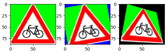
import cv2
import numpy as np
import matplotlib.pyplot as plt
img= cv2.imread('sign.png',cv2.IMREAD_COLOR)
img= cv2.cvtColor(img,cv2.COLOR_BGR2RGB)
h,w= img.shape[:2]
# Rotation using warpAffine
rM= cv2.getRotationMatrix2D((w/2,h/2),10,1) # Center, degrees, scale.
rimg= cv2.warpAffine(img,rM,(w,h),
                     orderMode=cv2.BORDER_CONSTANT,borderValue=(0,0,255))
# Perspective using warpPerspective - morph from start to target.
warpS= np.array([[0,0],[100,100],[0,100],[100,0]],np.float32)
warpT= np.array([[18,0],[100,100],[0,100],[82,18]],np.float32)
pM= cv2.getPerspectiveTransform( warpS, warpT )
pimg= cv2.warpPerspective(img,pM,(w,h))
# Plot
prows,pcols,fig= 1,3,plt.figure()
fig.add_subplot(prows,pcols,1)
plt.imshow(img)
fig.add_subplot(prows,pcols,2)
plt.imshow(rimg)
fig.add_subplot(prows,pcols,3)
plt.imshow(pimg)
plt.show()
A nonintuitive mapping function is cvCartToPolar and
cvPolarToCart. Why one would want to convert an image from Cartesian
coordinates to polar or the other way is a bit tricky. It is useful in
catching edge detection thresholds after other filtering is performed.
Another similar but weirder one is cvLogPolar. This transforms (x,y)
into (log radius,angle). If done just right, so the theory goes, this
provides a kind of invariance to planar rotation and scaling which
might be useful if trying to track an object. If the object scales,
its transform will shift on the horizontal. If the object rotates, the
transform will shift on the vertical. This might be useful, albeit
complicated, for tracking a fixed size moving object from a fixed
overhead camera.
OpenCV has cvDFT which is Discrete Fourier Transform. This is a
"fast" (FFT) O(N log N) version. Apparently, DFT is often overkill and
for practical situations a better function is likely to be cvDCT or
the Discrete Cosine Transform`.
Histogram
If an image is too dark or washed out, the variation between all the
pixels is not ideal in that it does not use the full range of
information expressible by the pixel value range. Plotting the
histogram of such an image will show most pixels concentrating in a
narrow band of value range. By using the cumulative distribution
function, the histogram can be remapped and the image revalued to make
sure that the resultant histogram uses more of the range. OpenCV has
the cvEqualizeHist function for this. While I can see this being
useful to improve the aesthetics of a rendered image for humans, I
wonder if it could really impart any more information to the image in
a way that would allow processing algorithms to actually do a better
job. In other words, what’s the difference between equalizing the
histogram and just having some feature recognition filter concentrate
only on a limited range of values?
But histograms have quite a few clever uses. Histograms of colors, edge gradients and other attributes can be used to determine scene specific content. Hand gesture recognition is one application. They can detect transitions in videos. Maybe a way to train a system to cut out ads. Hmm.
OpenCV has a lot of functions to make working with histograms as easy
and trouble-free as possible. Look for the data type CVHistogram and
the constructor/destructor functions cvCreateHist,
cvSetHistBinRanges, cvClearHist, and cvMakeHistHeaderForArray.
The last one uses data you have already organized to bless it as a
histogram that OpenCV can use.
Another way to generate less arbitrary and more mission oriented
histograms, is to automatically create them from images. The
cvCalcHist function can take an image and make a typical useful
histogram out of it involving a variety of properties.
Once the histogram is complete, accessing the data (or the pointer to
the data) can be achieved with functions such as cvQueryHistValue_nD
and cvGetHistValue_nD.
Also consider cvNormalizeHist which will replace values with the
portion of the total events that goes in that bin. So if you have 25
events and in bin x there are 5, the normalized form will replace the
5 with .2; everything should add up to 100% or 1 (though this can be
changed with the factor argument to the function).
Another valid approach which is subtly different is to normalize the
colors (or whatever) in your source data so that the histogram is
ready to be used with no further conditioning.
Another function to process the histogram is cvThreshHist that
basically resets bins with very few members. Imagine bins with counts
of 1,3,2,0,1,78,26,132,19,2,0,0,3,1. It is likely that thinking of
this data as 0,0,0,0,0,78,26,132,19,0,0,0,0,0 would be more useful.
The cvCopyHist function does the obvious but in several subtle
flavors involving either filling a pre-existing same size target
histogram with the source or creating (allocating) a target from
nothing.
The cvGetMinMaxHistValue gets minimum and maximum values obviously,
but how exactly isn’t entirely clear. I believe that it returns the
number of items in the bin with the most items and optionally the
index where that bin is. I don’t know how the latter part of that
handles ties.
Histograms can be compared with the cvCompareHist function. There
are several possible criteria, or "methods", which can be used.
-
Correlation. Perfect match = 1, total mismatch = -1, no correlation = 0.
-
Chi-square. Perfect match = 0, total mismatch = unbounded. Accuracy.
-
Intersection. Perfect match = 1, total mismatch = 0. Speed.
-
Bhattacharyya distance - a way to measure differences in statistical distributions which is sensitive to differences in mean and standard deviation. Perfect match = 0, total mismatch = 1. Accuracy.
There is another histogram comparing technique called
Earth Mover’s
Distance. This basically treats the items in bins as dirt that must
be moved and takes into account how much needs to be moved and how far
away to compare two probability distributions or histograms. OpenCV
has cvCaclEMD2 which is full of parameters allowing you to do fancy
things such as specify your own distance and work metrics.
Make sure to use cvNormalizeHist before comparing because comparing
unnormalized histograms is usually meaningless.
There is a technique called "back projection" which can determine how
well data fit the distribution of a histogram model. For example, if
you have a histogram of an object you can see if an image contains
regions with a similar histogram using back projection. The function
to consider is cvCalcBackProject. A related function is
cvCalcBackProjectPatch which will check if an image contains sub
regions that are well matched.
A similar thing is template matching which does similar things
to the histogram functionality but without histograms per se. This
uses cvMatchTemplate to take patches of image, say a thumbnail
sized image of just an apple, and scan a larger image looking for
likely similar regions. There are all kinds of similarity metrics as
is typical and they all have subtle functionality and performance
tradeoffs.
Contours
Contours are ways to manage features of images. They are stored as
CvSeq type sequences (linked-lists deep down). Contours can be
created from images filtered by cvCanny or cvThreshold, etc using
the cvFindContours function. This function can get tricky in the
same way a bucket fill tool can get tricky with respect to finding
islands on lakes on islands in lakes, etc (see 69.793° N, 108.241° W
for an example). OpenCV calls these things "contours" (islands) and
"holes" (lakes). This all apparently does often get quite complex and
OpenCV has a fancy data structure called a "contour tree" to organize
these complex relationships. In this structure, the world’s continents
(sticking with the geography metaphor) would have contours at the top
of a tree and all lakes would be children. And islands on those lakes
would be (contour) children of their respective lakes, ad infinitum.
Back in the world of image processing, the islands often have lakes
that match them exactly (like an atoll) because that’s how edge
detection filters. This means that edges tend to have inner and outer
edges themselves just as an atoll has an outer beach and an inner
beach, but the atoll separates the lagoon from the sea.
The cvFindContours function expects an 8-bit single-channel image
which, it is important to note, will be mangled during calculation
(make a copy if that’s needed). This function will allocate the
CvSeq structures necessary (and free them) but it’s a little
confusing how to set it up. The firstContour parameter takes a
pointer to a pointer that would point toward the first contour if
it existed. But it doesn’t because the function spawns it. But that
pointed to pointer is where you’ll find the head of the tree structure
that results from the function. The return value is the total number
of contours found. The mode and method parameters respectively specify
what sort of operation should be calculated and exactly how if there
are variants.
There are four different modes which basically specify the topology of the resulting tree of contours.
-
CV_RETR_EXTERNAL - simplistic, there’s one contour, no linked structures.
-
CV_RETR_TREE - island1’s child is a list of lake01 and lake02; lake01’s children is a list of island010 and island011, etc.
-
CV_RETR_CCOMP - a list of just contours, holes are doubly linked to the contours (the holes are in their own lists and their heads are tacked to the contour node).
-
CV_RETR_LIST - Get’s all contours and puts them in single list using
h_prevandh_next. This is by far the easiest to use and the default.
After figuring out how you want the contours to be organized internally, the next thing is to specify the technique used to compose the contours themselves. There are several and they’re pretty technical.
-
CV_CHAIN_CODE
-
CV_CHAIN_APPROX_NONE
-
CV_CHAIN_APPROX_SIMPLE - The default. Maybe best to start here.
-
CV_CHAIN_APPROX_TC89
-
CV_LINK_RUNS
To get an idea of what these things are, this might be helpful. Described simply, chain code starts with coordinates of a boundary pixel and then is a stream (or chain) of directions one would need to travel to stay on the boundary. When the original point is arrived at, the region is defined. The specific case of Freeman chains is an 8 direction system with 0 at 12 o’clock going to 7 at 10:30. This encoding doesn’t have to be at the pixel level and can be quite rough making it a very efficient way to describe large areas of input images.
Besides cvFindContours, there is another way to do things. There is
a cvStartFindContours which creates a "scanner" or a
CvSequenceScanner object. You can iterate over the contours with
cvFindNextContour. When finished, cvEndFindContour stops that
process.
An important utility is to be able to draw contours which can be done
with cvDrawContours. This allows all the normal stuff like line
color and thickness as well as the levels of the tree to plot.
A negative line thickness field (or set to CV_FILLED) will fill the
contour allowing for solid shapes. This can be useful for making masks
from vector paths (basically contours).
Here’s a Python example of drawing some simple shapes on an image.
roi= np.array( [(600,safe), (960,safe), (960,880), (50,1080)] )
cv2.drawContours(f, [roi], 0, (0,0,255), -1)
Once the contour has been found, you can use cvApproxPoly
on it to convert it to a contour with fewer points. This is basically
a raster to vector operation even though the result is still a contour
sequence. The algorithm works by finding maximally distant points on
the original contour. Those are the first two of the final points.
Then the line between them is checked to see where it is farthest from
the contour. That point on the contour is added to to new approximated
contour. This continues until the desired number of points is reached.
A related function is cvFindDominantPoints which seems very similar
to what I call "cull shallow angles" in to2d. It differs in that it
can look at several points away from just its immediate neighbor. It
is the same basic idea though i.e. to do what the function name
suggests. The method is selectable, but there is only one choice
CV_DOMINANT_IPAN. This IPAN stuff is stupidly named and should be
treated as a random label for this technique.
Now that you have simple or complex contour sequences, there are some
calculations you can do that can be informative. There is
cvArcLength and cvContourPerimeter. The former can provide lengths
of just portions of the contour (use slices). The cvContourArea is
similar and can also do a portion of the contour or you can set slice
= CV_WHOLE_SEQ.
Another useful thing to do with a contour sequence is to get an even
rougher idea of where it is by using cvBoundingRect. This is
parallel to the X and Y axes. If you want the truly smallest rectangle
regardless of orientation, check out cvMinAreaRect2 which returns a
type CvBox2D (containing center x and y, size x and y, and angle).
In the same spirit as the bounding box functions, there is also
cvMinEnclosingCircle. Related, but with a different approach is
cvFitEllipse2. This does not ensure the resulting ellipse contains
all points but rather does a kind of least squares fitting function.
After finding the contours and distilling them down to bounding boxes,
you can check for collisions and the like. The questionably named
cvMaxRect function takes 2 rectangles as input and returns a rect
(actually a CvRect) which is the smallest rectangle that will
enclose both.
Getting fancier is a function to calculate moments,
cvContourMoments which returns into a special data type,
CvMoments. It seem that function is actually a wrapper for the
cvMoments function which can provide normalized moments too. This
allows for comparing different sized objects in a consistent way. More
specialty functions are cvGetCentralMoment,
cvGetNormalizedCentralMoment, cvGetHuMoments (rotation invariant).
More details about image
moments. This kind of thing might be useful to build object
recognition profiles, maybe something like OCR where each letter has a
set of moments that identify it regardless of position, size or
rotation. OpenCV has a function to compare shapes in this way (even
calculating the moments on the way), cvMatchShapes.
Because this isn’t complex enough, there is another more detailed way
to compare contours than the summary statistics like moments. Looking
at the details of the contour paths themselves is done by constructing
a data structure called CvContourTree which is not the same as the
data structure that contains a (possibly linked list of a) set of
contours. This is a tree that represents a single contour’s shape in a
way that is more easily matched by hierarchical geometric features.
This can all be thought of in black box terms as just another way to
compare shapes based on geometry. The functions provided to do this
are cvCreateContourTree, cvContourFromContourTree, and
cvMatchContourTree.
Another way to summarize shapes for comparison/identification purposes
is to calculate the convex hull and look for the differences, called
the convexity defects. OpenCV has cvConvexHull2 and
cvConvexityDefects to facilitate this. Also cvCheckContourConvexity can
determine if a contour is already convex.
If hulls are not enough, there is yet another matching strategy called
pairwise geometrical histograms. This basically takes the Freeman
chain codes mentioned above and makes a histogram of the direction
changes (a CCH, chain code histogram). See cvCalcPGH for the
function to do this.
Motion Detection
It seems that a primary way to scan images or sequences of images is
to look at rows of pixels at a time. There is a function
cvInitLineIterator that sets this up and a macro
CV_NEXT_LINE_POINT that moves from pixel to pixel in the line. I
think it works something like this.
CvLineIterator iterator;
int iterator_size;
iterator_size= cvInitLineIterator(rawImage,pt1,pt2,&iterator,8,0);
for (int j=0; j<iterator_size; j++) { CV_NEXT_LINE_POINT(iterator); }
You can sample whole lines at a time saving yourself the point to
point loop with cvSampleLine.
Frame Differencing
A simple way that objects can be detected in a scene is to subtract
the pixels of a frame now from the values of pixels from a little
while ago. The function cvAbsDiff does this helpfully dealing in
absolute values so it doesn’t matter which way around you go. This
function takes 2 input frames, one now, one before, and an output
frame called "frameForeground". I’m not keen on the use of the word
"foreground". Imagine pointing a camera out a window whose frame and
curtains were in the shot. That window would be the foreground but the
points of interest if something moved outside of the window are
technically in the background. But just be aware that this is the
terminology. When using the cvAbsDiff function, it’s usually
sensible to cut off minor fluctuations which are generally noise and
to set the rest to 255. Do this with cvThreshold.
There are much fancier ways that can help with things like blowing leaves on a tree in an outdoor scene. This wouldn’t want to be regarded as an object of interest in motion. One approach is to use averaging. OpenCV can develop a running average for the values of each pixel and when large deviations from that occur, do something special.
OpenCV has an accumulation function cvAcc that can help accumulate
statistics about a series of pixel changes. This function basically
adds up the value of the pixel which can be used with the total number
of images to get the mean value. Another similar metric is to use
cvRunningAvg. The cvSquareAcc can be useful in calculating the
variance of pixels. Presumably this will be a metric of how wildly the
values are differing which could be very relevant to motion detection.
The cvMultiplyAcc is another one that can be used in such
applications.
For complex moving backgrounds (windy trees), the ideal thing is to fit a distribution to the data that is present in the previous frames. Since this could imply using a lot of memory, a complex but efficient approach is to use the same kinds of tricks used by compression algorithms; check out codebooks. These focus on the important pixels more than the boring ones. The pro tip here is to use HSV or YUV and not RGB when doing fancy things like this.
Image Repair
A nice function is cvInpaint which can fill in small (thin really)
details that have been messed up in an image. It reminds me of the
clone tool in Gimp. So if you have a photo with some thin writing on
it done in a paint program, for example, this function can really do a
good job of blending it away. It seems ideal for camera artifacts and
grainy footage.
Mean-Shift Segmentation
The function is cvPyrMeanShiftFiltering and uses the pyramid
structures. To me the results of this remind me of "posterization".
But the technical description is something like this.
Given a set of multidimensional data points whose dimensions are (x, y, blue, green, red), mean shift can find the highest density “clumps” of data in this space by scanning a window over the space.
Motion Tracking
Lots of heavy math packed into OpenCV for this.
-
Harris corner detection. And friends Shi and Tomasi.
-
SIFT is Scale Invariant Feature Transformation and is not included in OpenCV. Just noting it as a related topic. It is used heavily in photogrammetry (here are my notes). There seems to be a C++ implementation contained in MVE. This paper seems to be the foundation of the technique.
-
Horn-Schunk Calculates a dense optical flow which is a map of all the displacements made by each pixel over time. It assumes smoothness in the flow over the whole image. This is a dense flow mapping and considered kind of inefficient for most cases. It’s OpenCV function is
cvCalcOpticalFlowHS. -
Block matching algorithms involve subdividing the image into smaller blocks and trying to find those blocks in subsequent images. If found, track the motion vector. Simple, but perhaps not especially efficient. OpenCV’s function for this is
cvCalcOpticalFlowBM.
Feature Detection
OpenCV has a function called cvGoodFeaturesToTrack() which uses the
Shi Tomasi algorithm, computes the second derivatives using Sobel
operators, calculates the required eigenvectors, (whew!) and
simply, from our point of view, returns a list of points that should
be pretty good for tracking. This list contains points that you hope
to be able to find again in another frame of the video. For example,
an edge can be moving parallel to its orientation and the motion may
be undetectable. A good feature, like a corner is noticeable whenever
it moves in any direction. Highlighting a few especially amenable
points allows for "sparse", but sensible, optical flow mapping.
If for some reason you require more precision in feature detection
than the grid of pixels would imply, explore cvFindCornerSubPix. This
will do some fancy dot product trickery to try and isolate corners
even more precisely than the bitmap would seem to allow. This seems
applicable in calibration operations.
A good example of cvFindCornerSubPix that works with little fuss can
be found
here.
Lucas-Kanade
Lucas-Kanade (also "LK") is a sparse flow mapping technique. This was used in the worm motility project. Requires consistent brightness, small motions frame to frame, and "spacial coherence" (which I do not exactly understand).
OpenCV deals with Lucas-Kanade implementations in two ways.
There is the cvCalcOpticalFlowLK function which just calculates the
flow field where it can be calculated (0 where it can not be). And
there is pyramid based processing with cvCalcOpticalFlowPyrLK.
Basically you need to supply the points you want to track in
featuresA (from cvGoodFeaturesToTrack usually) and call the
function. When it returns, check the status array to see which points
were actually tracked successfully and then check featuresB to see
where they are now.
Mean-Shift and CAMshift Tracking
Mean shift is a technique for
locating the maxima of a density function. It seems to work by
specifying a window enclosing some points, calculating the center of
mass of the points, recentering the window there, and iterating until
the window no longer needs to move. Of course choosing this window
wisely is a tricky detail. OpenCV has cvMeanShift to facilitate
this process.
CAM is "continuously adaptive mean-shift. This allows for the window
to be resized as necessary to accommodate things like a subject
getting nearer and farther away from the camera. Its function is
cvCamShift.
The features that these algorithms track are usually colors, but they can really track the distribution of any kind of feature. For example, my first thought was to use feature detection and track the distribution of "pointy bits" or straight edges. That may or may not work but it is theoretically possible with this framework.
Motion Templates
This technique to track motion relies on an initial silhouette being
specified. This could be done with chroma key or difference
calculations with a stationary camera or some other obvious technique.
You can also try some fancy technique like segmentation. A motion
history image (mhi) is created by setting the value of the output to the
current time stamp. Subsequent frames continue this and the older
images leave a fading trail of previous location ghosts. The function
cvUpdateMotionHistory helps with this.
By taking the gradient of this motion history map, perhaps by using
Scharr or Sobel techniques, the motion vectors can be ascertained.
OpenCV has cvCalcMotionGradient to get the gradients and
cvCalcGlobalOrientation to find the overall vector of motion, i.e.
the sum of the gradient vectors. Thinking of things like tracking a
single rotation invariant object like a billiard ball from a
stationary overhead camera, this is enough. But if you want to track
many balls, you’ll need to segment the motion profile with something
like cvSegmentMotion. This kind of complex technology could be
useful for gesture recognition, for example.
Estimators and Kalman Filtering
A Kalman filter is a mathematical process that forms ever better predictive models based on continual (though possibly discrete) input updates. It can be thought of as a type of sensor fusion as it can handle multiple indicators about a state. For example, GPS and odometry can be used as inputs and the more stable of these will contribute more (or something like that). In motion tracking this can take many input indicators of motion like the motion vectors calculated as above and integrate them to form a more stable and correct impression of the actual motion of the entire object of interest (not just its corners in isolation).
OpenCV provides a CvKalman data structure. It is created and
released with cvCreateKalman and cvReleaseKalman. The iterative
process of the Kalman cycle is executed with the functions
cvKalmanPredict and cvKalmanCorrect (those two functions provide
the best two word description of this complex technique).
The Kalman filter assumes that the uncertainty in the feedback is
Gaussian. That need not be the case. If there is a known bias, the
probability distribution can be represented as a density map (more
dense "particles" represent greater likelihood). This map with an
arbitrarily complex probability profile can be given to the the
cvCreateConDensation function which works much like the Kalman
functions.There is a CvConDensation struct like the CvKalman. The
tricky bit to using this is that this confidence map of particles
needs to be continuously updated to reflect known conditions. There is
no automatic way to do this.
Camera Calibration
I did extensive analysis into best practices for calibrating camera distortion. See my full post on the topic for details and a calibration program which exhaustively searches calibration images for detected points. The general strategy follows.
Cameras are not perfect and dealing sensibly with distortions caused by lens design and defects is critical to converting pixels received into meaningful knowledge about the real world’s geometry. The two types of systemic distortions that OpenCV helps with are radial and tangential. Radial distortions occur because the light deflection near the center of the lens is different than near the perimeter. Tangential distortion is a property of the image plane onto which the lens projects being not exactly aligned with the lens' proper axis.
OpenCV uses a "camera intrinsics matrix" and a "distortion vector" to
make adjustments. Figuring these out seems the tricky bit since once
they are established OpenCV can make corrections.
The cvCalibrateCamera2 helps figure out the correction data. It
looks at a reference specimen of known points from multiple views. It
also rotates to cross check. The reference specimen is usually a
chessboard patter and cvFindChessboardCorners can help with that
kind of target. It seems that after using that function to find the
chessboard points, it’s good to further refine the model with
cvFindCornerSubPix. To check you’ve got the right thing, there is
cvDrawChessboardCorners.
Once the chessboard is seen properly, a planar homography matrix is
needed that can convert between images and real locations which may be
in the shot at an angle or rotated. This can be done with
cvFindHomography. Once this is done actual camera calibration
(finding the distortions of the camera itself) are possible. This is
when cvCalibrateCamera2 is called.
Once you have the camera intrinsics and you just need to compute the
location of the objects in the scene. The
cvFindExtrinsicCameraParams2 function can take the intrinsic matrix
and the distortion coefficients that you have previously computed and
return a rotation and translation vector. Again this is all looking at
a known chessboard. So basically, you can use multiple views of a
chessboard to figure out what distortions are present in the optics of
the camera and from then on, you can look at a known fixed chessboard
in a scene and figure out where your camera is in space.
Once you have the the intrinsic matrix and distortion coefficients,
you probably want to correct the images. The functions
cvInitUndistortMap, cvUndistort2, and cvUndistortPoints all take
this data and rework an image to correct for the optical errors.
Simple Illustrative Example Programs
This test program should open the hard coded image and display it in a box.
#include <cv.h>
#include <highgui.h>

using namespace cv;
using namespace std;

int main(){
    Mat image;
    // Read the file
    image = imread("monkey.jpg", CV_LOAD_IMAGE_UNCHANGED);
    // Check for invalid input
    if(! image.data ){
        cout <<  "Could not open or find the image" << endl;
        return -1;
        }
    // Create a window for display.
    namedWindow( "Display window", CV_WINDOW_AUTOSIZE );
    // Show our image inside it.
    imshow( "Display window", image );
    waitKey(0);
    return 0;
    }
Here’s another similar minimal test doing things slightly differently.
#include "highgui.h"
int main( int argc, char** argv) {
    IplImage* img= cvLoadImage( argv[1] );
    cvNamedWindow("Example1", CV_WINDOW_AUTOSIZE );
    cvShowImage("Example1",img);
    cvWaitKey(0);
    cvReleaseImage(&img);
    cvDestroyWindow("Example1");
}
The same kind of thing for video.
#include "highgui.h"
int main(int argc, char** argv){
    cvNamedWindow("Example2", CV_WINDOW_AUTOSIZE);
    CvCapture* capture= cvCreateFileCapture(argv[1]);
    IplImage* frame;
    while (1){
        frame= cvQueryFrame( capture );
        if (!frame) break;
        cvShowImage( "Example2", frame);
        char c = cvWaitKey(33);
        if (c == 27) break;
    }
    cvReleaseCapture(&capture);
    cvDestroyWindow("Example2");
}
Camera Input
Using a camera is very similar to using a file. It just needs a camera number instead of a file name. Here’s an example of using a camera if no file is supplied.
#include "highgui.h"
int main(int argc, char** argv){
    CvCapture* capture;
    const char* title;
    if (argc==1) {
        capture= cvCreateCameraCapture(0);
        title= "Camera 0";
    } else {
        capture= cvCreateFileCapture(argv[1]);
        title= argv[1];
    }
    cvNamedWindow(title, CV_WINDOW_AUTOSIZE);
    IplImage* frame;
    while (1){
        frame= cvQueryFrame( capture );
        if (!frame) break;
        cvShowImage( title, frame);
        char c = cvWaitKey(33);
        if (c == 27) break;
    }
    cvReleaseCapture(&capture);
    cvDestroyWindow(title);
}
Filtered Video Feed With Controls
Here is a program that will open and display a camera feed, some control slider bars, and a feed of the resultant modified video. This allows one to adjust settings in real time to capture the best parameters to use in filtering work. This is handy in isolating particular objects of interest. See the video at the top. Some good parameters for the car (i.e. yellow highligher) are H=27-41, S=58-128, V=199-255.
#include <iostream>
#include <cv.h>
#include <highgui.h>
#include "opencv2/imgproc/imgproc.hpp"

using namespace cv;
using namespace std;

int main(int argc, char* argv[]) {
    // Open video file for reading.
    VideoCapture cap_ob(0);
    if (!cap_ob.isOpened()) {
        cout << "Cannot open the video file." << endl;
        return -1;
        }
    // Create a window for the controls.
    namedWindow("Control", CV_WINDOW_AUTOSIZE);
    // Define control ranges.
    int iLowH= 0; int iHighH= 179; // Hue (0-179)
    int iLowS= 0; int iHighS= 255; // Saturation (0-255)
    int iLowV= 0; int iHighV= 255; // Value (0-255)
    // Create trackbars in Control window.
    cvCreateTrackbar("Hue (min)","Control",&iLowH,179);
    cvCreateTrackbar("Hue (max)","Control",&iHighH,179);
    cvCreateTrackbar("Sat. (min)","Control",&iLowS,255);
    cvCreateTrackbar("Sat. (max)","Control",&iHighS,255);
    cvCreateTrackbar("Val. (min)","Control",&iLowV,255);
    cvCreateTrackbar("Val. (max)","Control",&iHighV,255);

    while (true) {
        Mat imgOriginal;
        // Read new frame from video.
        bool bSuccess= cap_ob.read(imgOriginal);
        if (!bSuccess) {
            cout << "Cannot read the frame from video file." << endl;
            break;
            }
        Mat imgHSV;
        // Convert from BGR to HSV.
        cvtColor(imgOriginal,imgHSV,COLOR_BGR2HSV);

        Mat imgFiltered;
        inRange( imgHSV,
                 Scalar(iLowH,iLowS,iLowV),
                 Scalar(iHighH,iHighS,iHighV),
                 imgFiltered );
        // Show thresholded image.
        imshow("Filtered Image",imgFiltered);
        imshow("Original Image",imgOriginal);
        // The 10 is msec to wait between frames unless ESC (27) is pressed.
        if (waitKey(10) == 27) {
            cout << "ESC pressed. Bye." << endl;
            break;
            }
        }
    return 0;
    }
Notes
Look at convexHull which would work well to take the white points and calculate a bounding hull. Also see the bounding box method just above this one.
Actually, look at minarea. The Python demo makes this clearly a candidate.
How to get the centroid of that thing? Maybe there’s a way to get the centroid from a collection of white points.
Is there something that calculates the mean of a collection of points (centroid but called "mean")?
The program fitline.py is pretty excellent too if the marker can be
long and narrow.
Misc
#include <iostream>
#include <cv.h>
#include <highgui.h>
#include "opencv2/core/core.hpp"
#include "opencv2/flann/miniflann.hpp"
#include "opencv2/imgproc/imgproc.hpp"
#include "opencv2/photo/photo.hpp"
#include "opencv2/video/video.hpp"
#include "opencv2/features2d/features2d.hpp"
#include "opencv2/objdetect/objdetect.hpp"
#include "opencv2/calib3d/calib3d.hpp"
#include "opencv2/ml/ml.hpp"
#include "opencv2/highgui/highgui.hpp"
#include "opencv2/contrib/contrib.hpp"
#include "opencv2/core/core_c.h"
#include "opencv2/highgui/highgui_c.h"
#include "opencv2/imgproc/imgproc_c.h"
PART TWO
Sorry about this mess. I had started taking a completely new set of notes as I read through the ORA Learning OpenCV book and they were growing quite extensive. And then I moved and I lost the notes! Dang! I just found them again and rather than update this nicely, I’m going to just dump the whole mess here to be sorted out properly later.
Build
A plausible Unix build command line for OpenCV programs.
gcc -v example2_2.cpp \
-I/usr/local/include/ -L/usr/lib/ -lstdc++ -L/usr/local/lib \
-lopencv_highgui -lopencv_core - -o example2_2
Other possible libraries which may be required to link to.
-
-lopencv_imgcodecs -
-lopencv_imgproc -
-lopencv_videoio -
-lopencv_video -
-lopencv_videostab
LD Path
export LD_LIBRARY_PATH=${LD_LIBRARY_PATH}:/opt/lib/Compile
g++ t.o /opt/lib/libopencv_highgui.so \
    /opt/lib/libopencv_core.so \
    /opt/lib/libopencv_imgcodecs.so -o t
Type
For the definitive place to learn more, check out this file:
opencv/cxcore/include/cxtypes.h
template class cv:Vec<> - used for small "fixed vector classes". I think it’s stuff like [x,y,z] kind of vectors and not STL type of vectors.
This has typedefs such as * cv::Vec2i - 2 integer member * cv::Vec3i - 3 integer members * cv::Vec4d - 4 double members * cv::Vec{2,3,4,6}{b,w,s,i,f,d} - any of these is valid
The fixed vector template cv::Vec<> is a cv::Matx<> whose number of columns is one.
The same setup is true for cv::Matx<> Also for small fixed 3x3 kind of matrices. Predefined size at compile time. * cv::Matx{1,2,3,4,6}{1,2,3,4,6}{f,d}
cv::Matx33f::all(.5); // Set all 9 (3x3) values to .5.
cv::Matx33f::zeros(); // Set all 9 (3x3) values to 0.
cv::Matx33f::ones(); // Set all 9 (3x3) values to 0.
cv::Matx33f::eye(); // 1,0,0,0,1,0,0,0,1 Identity
cv::Matx33f::randu(min,max); // Uniform random values.
cv::Matx33f::nrandn(mean,var); // Normally distributed random values.
m91f = m33f.reshape<9,1>(); // Cast to different dimensions.
m44f.get_minor<2, 2>( i, j ); // Sub matrix extraction.
m44f.row(i); // Isolate a row. Also `col`.
m44f.diag(); // Diagonal.
m44f.t(); // Tranpose.
m44f.inv(); // Invert.
m1.mul(m2) // m1[0][0]*m2[0][0], etc
Points could use the Vec templates, but they have their own class.
-
cv::Point{2,3}{i,f,d}
Unlike Vec, Points can use myP.x and myP.y, etc.
cv::Scalar is for 4 member doubles.
cv::Size has members width and height rather than x and y but is
similar to Point. cv::Rect has all four. There is cv::Size2{i,f} too
and cv::Size is really Size2i. There is cv::RotatedRect that contains
angle info too. sizeObj.area() is handy; works with Rect too.
rectObj.contains(pointObj) to check if point is in ROI.
Point Class
Some things that can be done with point classes.
cv::Point P;
cv::Point3f copyOfP(P);
cv::Point P2(x,y);
cv::Point P3(x,y,z);
P2.x=0,P3.z=0;
float dotProduct= P.dot(P2);
double doubleDotProduct= P.ddot(P2);
float crossProduct= P.cross(P2);
P.inside(R);
There is also a complex number class which is a lot like the STL complex<> template.
Range class
cv::Range class - contains start and end but end isn’t included. So
(0,5) means 0,1,2,3,4 but not 5. Method r.all provides the whole
list. r.size is the number of items provided (5 here).
Smart pointers
The smart pointer does reference counting for you. Create them like this.
-
cv::Ptr<Matx33f> p( new cv::Matx33f ) -
cv::Ptr<Matx33f> p= makePtr<cv::Matx33f>() -
cv::Ptr<IplImage> img_p( cvLoadImage("xed.png" ) ) -
cv::Ptr<IplImage> img_p = cvLoadImage( "xed.png" );
The magic here is that if a value of such a pointer object is assigned
to another variable, some behind the scenes bookkeeping goes on. For
example, if you have a smart pointer a and then you do b=a and
then some how get rid of a, it knows that b still needs it. Then
if b gets dropped, then it knows nothing cares about the referent
and it then calls destructors.
These cv:Ptr objects are like new smart_ptr<> template in fancy
new C++ versions. It’s also similar to the Boost shared_ptr<> smart
pointer.
Primative Templates
Trailing underscores are generally, but not always, indicate a template in OpenCV. Think of it as "FillInThe_".
These primatives are really just products of templates that can
actually be based on whatever types you want. So instead of using ints
in a cv::Point type you could use cv::Point_<int> or whatever type
you want as long as it supports basic operations. For example, the
complex number base could be used. This is mostly good to know to
understand error messages and how things work. Beyond that its usage
is exotic.
Utility Functions
Memory Related
-
cv::alignPtr()Align pointer to given number of bytes -
cv::alignSize()Align buffer size to given number of bytes -
cv::allocate()Allocate a C-style array of objects -
cv::deallocate()Deallocate a C-style array of objects -
cv::fastFree()Deallocate a memory buffer -
cv::fastMalloc()Allocate an aligned memory buffer
Math Related
-
cvCeil()a Round float number x to nearest integer not smaller than x -
cv::cubeRoot()Compute the cube root of a number -
cv::fastAtan2()Calculate two-dimensional angle of a vector in degrees -
cvFloor()Round float number x to nearest integer not larger than x -
cvIsInf()Check if a floating-point number x is infinity -
cvIsNaN()Check if a floating-point number x is “Not a Number” -
cvRound()Round float number x to the nearest integer
Output and Error Related
-
cv::format()Create an STL string using sprintf-like formatting -
cv::CV_Assert()Throw an exception if a given condition is not true -
CV_Error()Make a cv::Exception macro from a fixed string, throw it -
CV_Error_()Make a cv::Exception macro from a formatted string, throw it -
cv::error()Indicate an error and throw an exception
CPU, Threads, and Clock Ticks
-
cv::getCPUTickCount()Get tick count from internal CPU timer -
cv::getNumThreads()Count number of threads currently used by OpenCV -
cv::getThreadNum()Get index of the current thread -
cv::getTickCount()Get tick count from system -
cv::getTickFrequency()Get number or ticks per second (see -
cv::getTickCount() -
cv::setNumThreads()Set number of threads used by OpenCV -
cv::setUseOptimized()Enables SSE2 and other CPU optimizations -
cv::useOptimized()What CPU optimazations are in effect
Mat
The overwhelming majority of functions in the OpenCV library are
members of the cv::Mat class, take a cv::Mat as an argument, or return
cv::Mat as a return value; quite a few are and do all three.
This class is for "dense" matrices where every value is important.
Images are almost always dense. The data that each cell of one of
these objects holds can be chosen to suit the purpose. For example,
for a mask, it might be bool; for a color image it could be 3
channels of int.
Mat Constructors
cv::Mat; // Plain constructor.
cv::Mat( int rows, int cols, int type ); // Two-dimensional arrays with type.
cv::Mat( const Mat& mat, const cv::Rect& roi ); // ROI initialization.
cv::Mat( const Mat& mat, const cv::Range* ranges ); // ROI with ranges.
Mat Query
Here is an example of a 10x10 identity matrix with 32bit floating point numbers in one channel (grey maybe).
cv::Mat m= cv::Mat::eye( 10, 10, 32FC1 );Here is a way to access a value at the third row and 3rd column. Should be 1.00000.
printf( "Element (3,3) is %f\n", m.at<float>(3,3));If you want multichannel, the elements will be of Vec type so you’ll get channels at a certain point like this.
m.at<cv::Vec3f>(3,3)[0]Here is an example that calculates the longest element in a Mat. Actually, what it calculates is the sum of the squares of each channel and not really doing a great job remembering that.
int sz[3] = { 4, 4, 4 };
cv::Mat m( 3, sz, CV_32FC3 ); // Cube 4 positions long.
cv::randu( m, -1.0f, 1.0f );  // Fill random numbers (-1.0 to 1.0).

float max = 0.0f;              // minimum possible value of L2 norm

cv::MatConstIterator<cv::Vec3f> it= m.begin();
while( it != m.end() ) {
  len2 = (*it)[0]*(*it)[0]+(*it)[1]*(*it)[1]+(*it)[2]*(*it)[2];
  if( len2 > max ) max = len2;
  it++;
}
Ways to extract subsets of Mat objects. Note that these really create objects which point to the correct locations of the same actual data. To get a new manifestation of the actual data look into the copy function.
-
m.row(r) -
m.col(c) -
m.rowRange(start,end)- End might be the end element you want plus one. -
m.colRange(start,end)- Can also use cv::Range objects. -
m.diag(offset)- The diagonal of m. I think offset is optional. -
m( cv::Rect(x,y,w,h) );- ROI using Rect, can also use two cv:Range objects.
Matrix operations
-
m+n;m-n- addition and subtraction -
-m- matrix negation -
m+s;m-s- add or subtract from all elements -
m * sf- scale by a scale factor -
m0.mul( m1 );m0/m1- per element multiplication and division -
m*n- matrix multiplication -
m.inv()- invert matrix (optional methods for fancy people) -
m.t()- transpose matrix -
m>n;m>=n;m==n;m<=n;m<n- Per element comparison, returns uchar matrix b&w (0 or 255) -
m&n;m|n;m^n;~m- bitwise operations. Also against single values too -
min(m,n);max(m,n)- Single values work too -
cv::abs(m)- Absolute value of elements -
m.cross(n);m.dot(n); - Vector products (cross must be 3x1) -
cv::Mat::eye( r, c, t )- Make identity matrix with #rows and #cols of type t -
cv::Mat::zeros( r, c, t )- Make new matrix with all zeros -
cv::Mat::ones( r, c, t )- Make new matrix with all ones -
cv::norm()- ? Calculates normals vectors? -
cv::mean()- Scalar summary statistic, mean. -
cv::sum()- Scalar summary statistic, sum. -
n= m.clone()- deep copy a matrix -
m.copyTo(n)- deep copy a matrix, almost identical to clone() -
m.copyTo(n,mask)- deep copy a matrix only in masked locations -
m.convertTo(n,type,scale,offset)- change type, or enlarge,shrink, translate, etc. -
m.setTo(s[,mask])- set all or mask ROI to scalar value s -
m.reshape(channels,rows)- make i by j array something else -
m.push_back(s)- extend a 1d array with s (append), can tack rows on to 2d objects too -
m.pop_back(n)- pop n items off the end (note return is weirdly void) -
m.locateROI(size,offset)- ? region of interest help -
m.adjustROI(t,b,l,r)- ? region of interest help -
m.total()- count of elements -
m.elemSize()- size in bytes of each element including all channels -
m.elemSize1()- size in bytes of each element in each channel -
m.type()- what type is the Mat holding, int, float, etc -
m.depth()- number of channels -
m.size()- size of the whole m (I think) -
m.empty()- no elements are present.m.data()==NULL
cv::SparseMat
The cv::Mat is closely organized like C arrays because it is assumed that if you have 100 places, you’ll have 100 data points. But you may have a "sparse" situation where you have 100000 possible locations for 100 data points. The SparseMat class works almost like the Mat, but uses hash lookups instead of contiguous accounting. Some people think this has helpful functionality in vision problems in histograms.
Saturation casting - used to prevent over and underflows when doing math to values. For example if you double some int Mat and the values were already 200, they’ll overflow. In theory, as I understand it, this will set them to 255 and act like no problem.
Note on template vs. inheritance - while the primitive types are derived from their templates, the large array templates are instead derived from the basic class. There is some flexibility here but apparently it’s more proper to get a template to make you a class you need than to use templates for each thing in the class.
Helper Functions
-
cv::abs()- Return absolute value of all elements in an array. -
cv::absdiff()- Return absolute value of differences between two arrays. -
cv::add()- Perform element-wise addition of two arrays. -
cv::addWeighted()- Perform element-wise weighted addition of two arrays (alpha blending). -
cv::bitwise_and()- Compute element-wise bit-level AND of two arrays. -
cv::bitwise_not()- Compute element-wise bit-level NOT of two arrays. -
cv::bitwise_or()- Compute element-wise bit-level OR of two arrays. -
cv::bitwise_xor()- Compute element-wise bit-level XOR of two arrays. -
cv::calcCovarMatrix()- Compute covariance of a set of n-dimensional vectors. -
cv::cartToPolar()- Compute angle and magnitude from a two-dimensional vector field. -
cv::checkRange()- Check array for invalid values. -
cv::compare()- Apply selected comparison operator to all elements in two arrays. -
cv::completeSymm()- Symmetrize matrix by copying elements from one half to the other. -
cv::convertScaleAbs()- Scale array, take absolute value, then convert to 8-bit unsigned. -
cv::countNonZero()- Count nonzero elements in an array. -
cv::arrToMat()- Convert pre–version 2.1 array types to cv::Mat. -
cv::dct()- Compute discrete cosine transform of array. -
cv::determinant()- Compute determinant of a square matrix. -
cv::dft()- Compute discrete Fourier transform of array. -
cv::divide()- Perform element-wise division of one array by another. -
cv::eigen()- Compute eigenvalues and eigenvectors of a square matrix. -
cv::exp()- Perform element-wise exponentiation of array. -
cv::extractImageCOI()- Extract single channel from pre–version 2.1 array type. -
cv::flip()- Flip an array about a selected axis. -
cv::gemm()- Perform generalized matrix multiplication. -
cv::getConvertElem()- Get a single-pixel type conversion function. -
cv::getConvertScaleElem()- Get a single-pixel type conversion and scale function. -
cv::idct()- Compute inverse discrete cosine transform of array. -
cv::idft()- Compute inverse discrete Fourier transform of array. -
cv::inRange()- Test if elements of an array are within values of two other arrays. -
cv::invert()- Invert a square matrix. -
cv::log()- Compute element-wise natural log of array. -
cv::magnitude()- Compute magnitudes from a two-dimensional vector field. -
cv::LUT()- Convert array to indices of a lookup table. -
cv::Mahalanobis()- Compute Mahalanobis distance between two vectors. -
cv::max()- Compute element-wise maxima between two arrays. -
cv::mean()- Compute the average of the array elements. -
cv::meanStdDev()- Compute the average and standard deviation of the array elements. -
cv::merge()- Merge several single-channel arrays into one multichannel array. -
cv::min()- Compute element-wise minima between two arrays. -
cv::minMaxLoc()- Find minimum and maximum values in an array. -
cv::mixChannels()- Shuffle channels from input arrays to output arrays. -
cv::mulSpectrums()- Compute element-wise multiplication of two Fourier spectra. -
cv::multiply()- Perform element-wise multiplication of two arrays. -
cv::mulTransposed()- Calculate matrix product of one array. -
cv::norm()- Compute normalized correlations between two arrays. -
cv::normalize()- Normalize elements in an array to some value. -
cv::perspectiveTransform()- Perform perspective matrix transform of a list of vectors. -
cv::phase()- Compute orientations from a two-dimensional vector field. -
cv::polarToCart()- Compute two-dimensional vector field from angles and magnitudes. -
cv::pow()- Raise every element of an array to a given power. -
cv::randu()- Fill a given array with uniformly distributed random numbers. -
cv::randn()- Fill a given array with normally distributed random numbers. -
cv::randShuffle()- Randomly shuffle array elements. -
cv::reduce()- Reduce a two-dimensional array to a vector by a given operation. -
cv::repeat()- Tile the contents of one array into another. -
cv::saturate_cast<>()- Convert primitive types (template function). -
cv::scaleAdd()- Compute element-wise sum of two arrays with optional scaling of the first. -
cv::setIdentity()- Set all elements of an array to 1 for the diagonal and 0 otherwise. -
cv::solve()- Solve a system of linear equations. -
cv::solveCubic()- Find the (only) real roots of a cubic equation. -
cv::solvePoly()- Find the complex roots of a polynomial equation. -
cv::sort()- Sort elements in either the rows or columns in an array. -
cv::sortIdx()- Serve same purpose as cv::sort(), except array is. unmodified and indices are returned. -
cv::split()- Split a multichannel array into multiple single-channel arrays. -
cv::sqrt()- Compute element-wise square root of an array. -
cv::subtract()- Perform element-wise subtraction of one array from another. -
cv::sum()- Sum all elements of an array. -
cv::theRNG()- Return a random number generator. -
cv::trace()- Compute the trace of an array. -
cv::transform()- Apply matrix transformation on every element of an array. -
cv::transpose()- Transpose all elements of an array across the diagonal.
…6. Drawing == Drawing Properties === Colors * Normally 3 channels of cv:Scalar objects * 1st channel used when applied to 1 channel images * 4th channel tolerated but no alpha blending currently supported
Style
Note that "style" is not an OpenCV word per se.
* thickness - pixels thick as an integer. Or cv::FILLED for closed shapes.
* lineType - Either 4 or 8 or cv::LINE_AA. 4 and 8 are like
Minecraft placement where you can either only move orthoganally (4
possibilities) or on diagonals (8 possibilities). AA is
anti-aliasing.
Drawing Functions
-
cv::rectangle()- Ordinary rectanglevoid rectangle( cv::Mat& img, // Image to be drawn on cv::Point pt1, // First corner of rectangle cv::Point pt2 // Opposite corner of rectangle const cv::Scalar& color, // Color, BGR form int lineType = 8, // Connectedness, 4 or 8 int shift = 0 // Bits of radius to treat as fraction ); void rectangle( cv::Mat& img, // Image to be drawn on cv::Rect r, // Rectangle to draw const cv::Scalar& color, // Color, BGR form int lineType = 8, // Connectedness, 4 or 8 int shift = 0 // Bits of radius to treat as fraction );
-
cv::circle()- Ordinary round circles -
cv::ellipse()- Ellipses, whole or arcs, aligned or tilted, specified with normal details or cv::RotatedRect -
cv::fillConvexPoly()- Filled versions of simple polygons. Fast. Input points are sequential. Can’t figure 8 or otherwise cross. -
cv::fillPoly()- filled versions of arbitrary polygons. Can’t see the difference between this andthickness= cv::FILLED. -
cv::line()- Ordinary linevoid line( cv::Mat& img, // Image to be drawn on cv::Point pt1, // First endpoint of line cv::Point pt2 // Second endpoint of line const cv::Scalar& color, // Color, BGR form int lineType = 8, // Connectedness, 4 or 8 int shift = 0 // Bits of radius to treat as fraction );
-
cv::polyLines()- Multiple polygonal curves. Assumed open unlessisClosed=truevoid polyLines( cv::Mat& img, // Image to be drawn on const cv::Point* pts, // C-style array of arrays of points int npts, // Number of points in 'pts[i]' int ncontours, // Number of arrays in 'pts' bool isClosed, // If true, connect last and first pts const cv::Scalar& color, // Color, BGR form int lineType = 8, // Connectedness, 4 or 8 int shift = 0 // Bits of radius to treat as fraction );
-
cv::clipLine()- Determine if a line is inside a given box -
cv::ellipse2Poly()- Approximation function for breaking down true mathematical ellipses into something plottable.
Text
cv::putText()
void cv::putText(
  cv::Mat&      img,                      // Image to be drawn on
  const string& text,                     // write this (often from cv::format)
  cv::Point     origin,                   // Upper-left corner of text box
  int           fontFace,                 // Font (e.g., cv::FONT_HERSHEY_PLAIN)
  double        fontScale,                // size (a multiplier, not "points"!)
  cv::Scalar    color,                    // Color, RGB form
  int           thickness = 1,            // Thickness of line
  int           lineType  = 8,            // Connectedness, 4 or 8
  bool          bottomLeftOrigin = false  // true='origin at lower left'
);
All fonts are based on Hershey vector fonts.
|
Normal size sans-serif |
|
Small size sans-serif |
|
Normal size sans-serif; more complex than cv::FONT_HERSHEY_SIMPLEX |
|
Normal size serif; more complex than cv::FONT_HERSHEY_DUPLEX |
|
Normal size serif; more complex than cv::FONT_HERSHEY_COMPLEX |
|
Smaller version of cv::FONT_HERSHEY_COMPLEX |
|
Handwriting style |
|
More complex variant of cv::FONT_HERSHEY_SCRIPT_SIMPLEX |
Also cv::FONT_HERSHEY_PLAIN | cv::FONT_HERSHEY_ITALIC
cv::getTextSize() - calculates how big text would be. Only in Y?
Random Numbers
OpenCV provides special functor objects, one of which provides random number generation services (PCA-Priciple Component Analysis and SVD-Singluar Value Decomposition are others).
Every thread gets its own random number generator object. You can access it like this.
cv::RNG rng = cv::theRNG();Then make use of it with.
cout << "An integer: " << (int)rng   << endl;
cout << "A float:    " << (float)rng << endl;
Besides matrix methods that incorproate these objects, there are direct methods to do things. Some examples.
-
cv::RNG::uniform
-
cv::RNG::gaussian
-
cv::RNG::fill
HighGUI - In OpenCV3 it is now broken up.
-
imgcodecs.hpp
-
videoio.hpp
-
highgui.hpp (includes imgcodecs.hpp and videoio.hpp)
Also has some XML/YML features for saving parameters and data, etc.
Load Images With Read
cv::Mat cv::imread( const string& filename, int flags);
Default flags is cv::IMREAD_COLOR
three 8-bit channels.
|
3 |
|
1 |
|
1-3 |
The cv::IMREAD_ANYDEPTH flag can allow greater than 8-bit channels.
The flag cv::IMREAD_UNCHANGED combines ANYCOLOR and ANYDEPTH to try
to exactly match whatever is in the file no matter what it is.
imread looks at the file itself and does not trust any filename
conventions like jpegimagesendwith.jpg.
If the read fails there is no error but the resulting image will be
empty. You can check with cv::Mat::empty()==true.
Save Images With Write
bool cv::imwrite(const string& fn, cv::InputArray img, const vector<int>& params=vector<int>());This takes the file name string and an image array and writes the file. The final parameter is optional and is used to control things like PNG compression (default 3) or JPEG quality (default 95).
Reading Video Streams
This opens a video file.
cv::VideoCapture::VideoCapture( const string& fn,);This opens a camera device. The first is 0.
cv::VideoCapture::VideoCapture( int device );I think that a device of 200 is the first V4L (video4linux) device,
201, the 2nd, etc. 300 is the first firewire device. 500 is the first
QT device. But 0 is the first of any found (cv::CAP_ANY).
You can check that it opened properly and is ready to go with this.
cv::VideoCapture::isOpened()==trueTo read a frame.
bool cv::VideoCapture::read(cv::OutputArray image);The image will be empty and the return false if the read did not go
well or you have come to the end of the file, i.e. last frame.
There’s an alias to the >> but that seems more, not less, complex to
me. Speaking of complex, the read operation can also be broken down
into a cv::VideoCapture::grab and a cv::VideoCapture::retrieve
sequence. This can be handy to "grab" from multiple cameras as close
to simultaneously as possible, then do more time consuming decoding on
the input. This allows triangulation and stereo analysis to minimize
error.
Video Metadata
The cv::VideoCapture::get() and cv::VideoCapture::set() functions
allow access to the metadata contained in some video file formats.
Handy things to query could be…
-
cv::CAP_PROP_FRAME_WIDTH -
cv::CAP_PROP_FRAME_HEIGHT -
cv::CAP_PROP_FPS -
cv::CAP_PROP_FOURCC- Four character code of the codec involved -
cv::CAP_PROP_FRAMECOUNT
There are many others, not all of which are reliably available for every codec.
Writing Video
First you need a writer object. This gives you a chance to set what the output properties will be like.
cv::VideoWriter::VideoWriter( const string& filename, int fourcc, double fps,
                              cv::Size frame_size, bool is_color=true );
Here are typical settings showing how to update the object too.,
cv::VideoWriter out;
out.open("vid.mpg", CV_FOURCC('D','I','V','X'), 30.0, cv::Size( 640, 480 ), true);
if (out.isOpened() == true) { out.write(const Mat& image) }
This creates an MPEG-4 codec, with 30 fps, 640x480 size, expecting
only color. The CV_FOURCC function handles bit packing to form the
weird codec codes used in this business. As with the read the
cv::VideoWriter::write() funciton has an analogue with << which I
also think is overly complex. But good to recognize.
Object Serialization And Persistence
OpenCV also has ways to write various non image objects to files in key/value formats. This could be handy for parameter sets. Basically look into this sort of thing.
cv::FileStorage fs("test.yml", cv::FileStorage::WRITE);This will open an object fs which will write objects as YML. It
works something like this.
fs << "Contrast" << mycontrast;Retrieve the data in these files with something like this. (Didn’t check it.)
mysettingsfile= open("test.yml", int flag);
int contrast;
mysettingsfile["Contrast"] >> contrast;
I am pretty sure XML is supported too.
GUI Windows
GUI windows pretty much are for showing images. OpenCV does not return a window object as one would expect. This is how windows the lifecycle of a window is handled.
int cv::namedWindow( const string& name, int flags );
void cv::imshow( const string& name, cv::InputArray image );
int cv::destroyWindow( const string& name );
void cv::destroyAllWindows( void );
Instead of handling the window with an object, you refer to it by its
name string. I think this is designed to be awkward enough so that
people don’t start building truly fancy things with OpenCV. The flags
can be 0 which means let users resize or it can be
cv::WINDOW_AUTOSIZE which conforms to a loaded image automatically.
When the image is applied to the window it gets its own buffer so that
changes to the window’s base image are not reflected until a new call
to imshow.
int cv::waitKey( int delay );If and only if a window is successfully open, the waitKey function
will wait for a UI keypress event. The delay is the time in
milliseconds until it gives up waiting and just proceeds onto the next
command (0 means do not time out). If the function does time out it
returns a -1.
Here a simple example that shows the file provided as an argument until the user presses escape (character 27). The file name is used to refer to the window and is displayed in its title bar.
int main( int argc, char** argv ) {
    cv::namedWindow( argv[1], 1 );
    cv::Mat = cv::imread( argv[1] );
    cv::imshow( argv[1], img );
    cv::moveWindow( argv[1], 0, 0); // Set upper left to 0,0.
    while( true ) { if( cv::waitKey( 100 ) == 27 ) break; }
    cv::destroyWindow( argv[1] );
    exit(0);
}
For proper operating systems there is also this mysterious command.
int cv::startWindowThread( void );This, in theory, allows OpenCV to start a separate thread for a windoow (each extant window?) allowing it to respond better even while other things are going on.
Mouse Events
Working with mouse events requires a callback. The function must look something like this prototype.
void mouse_cb( int event, int x, int y, int flags, void* param );Here event and flags are codes refering to these actions and circumstances.
-
cv::EVENT_MOUSEMOVE
-
cv::EVENT_LBUTTONDOWN
-
cv::EVENT_RBUTTONDOWN
-
cv::EVENT_MBUTTONDOWN
-
cv::EVENT_LBUTTONUP
-
cv::EVENT_RBUTTONUP
-
cv::EVENT_MBUTTONUP
-
cv::EVENT_LBUTTONDBLCLK
-
cv::EVENT_RBUTTONDBLCLK
-
cv::EVENT_MBUTTONDBLCLK
-
cv::EVENT_FLAG_LBUTTON
-
cv::EVENT_FLAG_RBUTTON
-
cv::EVENT_FLAG_MBUTTON
-
cv::EVENT_FLAG_CTRLKEY
-
cv::EVENT_FLAG_SHIFTKEY
-
cv::EVENT_FLAG_ALTKEY
The x and y coordinates are where the mouse action happened. I believe it is in the coordinate system of the image matrix, not the entire user desktop, but I’m not 100% sure. I also don’t know why the events and flags seem to have redundant coverage of the mouse buttons. The param argument is a pointer that allows this callback to pass back any kind of thing as a pointer.
Once you have a mouse action to perform ready in the callback function, you need to register that callback to hook it up to the proper window.
void cv::setMouseCallback( const string& windowName,
     cv::MouseCallback mouse_cb, void* param = NULL );
Trackbars
int cv::createTrackbar( const string& trackbarName,
    const string& windowName, int* value,int count,
cv::TrackbarCallback onChange=NULL, void* param=NULL );-
trackbarName - Handle used to identify trackbar
-
windowName - Handle used to identify window == NEXT - Chapter 9.2
-
value - Slider starting setting and pointer which will be updated by trackbar events.
-
count - Total counts for slider at far right, or max value.
-
onChange - Callback function (optional)
-
param - Additional params for callback fn (if any).
If you want to use a trackbar event callback, here is the prototype.
void a_tb_cb( int tb_pos, void* param=NULL );Here are two functions that allow you to query and change the state of the trackbar (supply an identifying window name and trackbar name).
int cv::getTrackbarPos( const string& tb,const string& win);
void cv::setTrackbarPos( const string& tb,const string& win,int pos);
QT
HighGUI basically reinvents functionality for every platform it supports. Another way that’s gaining popularity is to use QT for HighGUI’s backend. This means that the cross platform part is handled by QT developers. Here’s a summary of the situation.
-
Native HighGUI - Custom coded to the architecture.
-
QT backend HighGUI - OpenCV HighGUI extended to architectures with QT backend. To suppress any fancy features of this and emulate classic native HighGUI, add the
cv::GUI_NORMALflag to thecv::namedWindow()call. You may needcv::GUI_EXTENDEDfor those fancy features. Seems not consistent across platforms. -
QT - OpenCV does not use its own GUI at all. GUI requirements are all met by QT and OpenCV just manipulates the data.
With extended or normal GUI, if you’re using the QT backend you can also put a text overlay on images. This is the function to use.
int cv::displayOverlay( const string& winname, const string& text, int delay );Use delay of 0 for indefinite, otherwise the overlay text is temporary.
There is also a "statusbar" for QT backend GUI windows. This is not the title bar. This is just a line of text under the image. I think it kind of wastes space, but here it is.
int cv::displayStatusBar( const string& winname, const string& text, int delay );Same rules as the overlay.
The QT GUI backend has another fancy feature where every application
(not each window) has a "properties" system that can be accessed with
the icon that looks (to me) like a whisk broom. Track bars can be put
here so they are normally out of the way. To put trackbars into this
system, just leave the name blank (i.e. "") when specifying the window
to attach the trackbar to in the createTrackbar call.
Unlike native HighGUI, QT HighGUI also features buttons. int cv::createButton( const string& buttonName, cv::ButtonCallback buttonCB = NULL, void* params, int buttonType = int, initialState = 0);
The buttonName will label the button; leave it blank and it will get labeled 0,1,2, etc.
The buttonType is either cv::PUSH_BUTTON, cv::CHECKBOX, or cv::RADIOBOX. The callback that the button press triggers looks like this.
void buttonCB( int state, void* params );For fancy fonts using QT HighGUI, look into the CvFont object returned from the cv::fontQt() function. Then add fancy text with cv::addText().
QT HighGUI also allows some window properties to be queried and even modified. This seems important when considering windowed mode vs. full screen. See cv::getWindowProperty and cv::setWindowProperty. You can also save and then later reload the state of all your window locations and GUI element settings. See cv::saveWindowParameters and cv::loadWindowParameters. The magic of how this happens is opaque to the user/programmer, but note that it depends on the executable name so if you change that, be prepared.
QT HighGUI also can register a callback to draw OpenGL buffers into the OpenCV GUI elements. Do this with cv::createOpenGLCallback.
Image Processing
Image Border Padding
To apply a NxN kernel to an image it’s clear that at certain edge pixels N/2+1 of the kernel will hang off the edge. This can be handled by cropping down the final image. Or you can pad out the original image with a synthetic border. There are many modes in OpenCV to do this.
void cv::copyMakeBorder( cv::InputArray srcimg, cv::OutputArray dstimg, int t_pad, int b_pad, int l_pad, int r_pad, int borderType, const cv::Scalar& value=cv::Scalar() );
The value is for constant (e.g. all black or white or greenscreen) borders. The borderType can be one of the following.
|
Soild color frame effect. |
|
Toroidal. |
|
Use value of edge pixel. (Corner?) |
|
Frame is a reflection of edge. 654321 becomes 456-654321-123 |
|
Reflect without double wide edge pixel. 345-654321-234 |
|
Same as cv::BORDER_REFLECT_101. |
Threshold
To selectively apply a filter based on some kind of single per pixel
operation, the cv::threshold function can do that. It takes a source
and destination array and the threshold values.
double cv::threshold( cv::InputArray S, cv::OutputArray D,
                      double threshValue, double maxValue, int thresholdType  );
|
Dij = (Sij > threshValue) ? maxValue : 0 |
|
Dij = (Sij ⇐threshValue) ? maxValue : 0 |
|
Dij = (Sij > threshValue) ? Sij : 0 |
|
Dij = (Sij ⇐threshValue) ? Sij : 0 |
|
Dij = (Sij > threshValue) ? threshValue : Sij |
The threshValue can also be cv::THRESH_OTSU. This will make the
threshold() function try to find the optimal threshold value. This
maximizes the variance between the separated sets of pixels.
This is a relatively slow function.
There is also the adaptive threshold function. This is the same technique that boosts the performance so much in findChessBoardCorners.
void cv::adaptiveThreshold( cv::InputArray src, cv::OutputArray dst,
     double maxValue, int adaptiveMethod, int thresholdType int blockSize,
     double Constant );
The threshold value is computed on the fly for each pixel based on a weighted average of a (blockSize2 - Constant) region around it. The adaptiveMethod parameter is either "mean" or "Gaussian" (cv::ADAPTIVE_THRESH_MEAN_C or cv::ADAPTIVE_THRESH_GAUSSIAN_C). Gaussian gives wieghted values while mean is constant for that region.
Smoothing
There are at least 5 different kinds of smoothing operation in OpenCV.
The simplist is cv::blur().
void cv::blur( cv::InputArray  src, cv::OutputArray dst,
           cv::Size kernelSize, cv::Point anchorPt=cv::Point(-1,-1),
           int borderType=cv::BORDER_DEFAULT);
This just takes a kernelSize kernel and computes the mean value within
it. This is the value assigned to the new image at the location the
kernel was centered on. Since the kernel is rectangular this is a
generalization of a "box filter". The cv::boxFilter() function is a
more general case of cv::blur which allows for unnormalized mode and
an explicit control over output depth (blur reasonably assumes
normalizing and same depth).
Here is another similar kind of blur which uses the median of the
kernel’s contents rather than the mean as with simple blur. It seems
to me to lose most detail, but if you want major component
segmentation, it migth be ideal.
void cv::medianBlur( cv::InputArray src, cv::OutputArray dst, cv::Size kernelSize );Ths GaussianBlur is a much nicer looking function which produces results that are what you’d expect with wearing the wrong glasses. Detail can be preserved while noise can be muted.
void cv::GaussianBlur( cv::InputArray  src, cv::OutputArray dst, cv::Size kernelSize,
                       double sigmaX, double sigmaY=0.0, int borderType=cv::BORDER_DEFAULT);
The sigmaX and sigmaY are "Gaussian half-width" in each direction.
What that means is vague but I assume it has to do with the shape of
the Gaussian probability distribution used, perhaps related to the
variance. If you leave it at 0, it will, in theory, used optimized
code. Also 3, 5, and 7 square kernels get special hand tuned
opmization boosts. See Image Border Padding for how to handle borderType.
The other type of smoothing is bilateral filtering. You can think of this as Gaussian smoothing that weighs similar pixels more highly than less similar ones, keeping high-contrast edges sharp.
void cv::bilateralFilter( cv::InputArray src, cv::OutputArray dst,
      int d, double sigmaColor, double sigmaSpace,
            int borderType=cv::BORDER_DEFAULT );
The d is distance to consider (sort of like a kernel, but I think it really computes expensive distances). Some sources call this a "diameter" which is a different thing but I guess it has the same rough effect when adjusting it. The sigmaColor is like the sigmas for Gaussian blur. The sigmaSpace affects what will be included in the smoothing; the larger it is, the more extreme a discontinuity must be to be preserved.
Derivatives and Gradients
A derivative is the rate of change of a process. So if I have a value of 9 and then 9 and 9 and 9, the derivative is 0 because it’s not changing at all. If I have a value of 3, then 6, then 9 then 12, the derivative is 3. This is of interest in image processing because if you have pixels with the following values, [7,9,8,10,9,54,53,54,53,55], it’s easy to see that in the middle of that sequence something important happened. In this sequence the derivatives are [2,-1,2,-1,45,-1,1,-1,2] and by plotting this, you get a representation of the edges. This is a simplification; in practice the derivative functions often will be fitting polynomials and other fancy things in the internals.
Sobel
The least fancy edge detection is the Sobel derivative.
void cv::Sobel( cv::InputArray, cv::OutputArray, int ddepth,
  int xorder, int yorder, cv::Size kernelSize=3,
  double scale=1, double delta=0, int borderType=cv::BORDER_DEFAULT);
The ddepth can change to output’s format (to CV_8U) for example)
which is handy since your image of the edges doesn’t need all the
color info of the original. The kernel size should be odd but not
exceed 31. The order is the derivative order, presumably 1st
derivative (1) for normal gradients. Second order (2) is also an
option and even zero, though I don’t know what that means exactly in
this context. Scale and offset are applied to values before
calculation to help put the result in a usable (visible maybe) range.
Scharr and Laplacian Variants
The Sobel filter has better performance the closer the edge aligns
with horizontal or vertical. To help with that, for example to
improve the accuracy of histogram of oriented gradients approaches,
you can use the special kernelSize parameter of cv::SCHARR. This
will create a (fast) 3x3 kernel that is more balanced for edges in any
oreintation.
The cv::Laplacian() function (not to be confused with the Laplacian
pyramid) is basically the cv::Sobel() with order set to 2. This can
be useful for edge detection. It looks like it favors strong
distinctions and ignores milder gradient changes.
Morphology
This kind of operation is important for removing noise and clarifying object definition. The two basic transforms are dilation and erosion. Dilation adds active pixels around currently active pixels while erosion does the opposite. Dilation tends to fill holes and concave features while erosion tends to smooth out jagged protrusions. Both functions take basically the same kinds of parameters.
void cv::dilate/cv::erode( cv::InputArray src, cv::OutputArray dst, cv::InputArray kernel, cv::Point anchor=cv::Point(-1,-1), int iterations=1, int borderType=cv::BORDER_CONSTANT, const cv::Scalar& borderValue=cv::morphologyDefaultBorderValue() );
Both src and dst can be the same. The kernel supplied with an
uninitialized cv::Mat() will give the default 3x3. These functions
are really just different directions of focus, either on lightening or
darkening.
These morphology functions are usually fine for 1 bit image masks. For
fancier applications on more complex image arrays, you might want a
more complex general morphology functionality. This is the purpose of
the cv::morphologyEx() function. Some odd terminology in this topic
is "top hat" and "black hat" which basically are techniques to isolate
patches that are brighter or dimmer, respectively, mostly in grayscale
work.. You can also make your own wierd fancy kernel shapes using
cv::getStructureElement but that’s pretty exotic. In fact, you can
delve into the internals of these 2d filters (cv::filter2D()) and
use subcomponents of OpenCV’s mainstream functions to compose your own
optimized solution.
Image Transforms
Probably the most essential general image transform is cv::resize
which does the obvious.
void cv::resize( cv::InputArray src, cv::OutputArray dst, cv::Size dsize,
  double fx=0, double fy=0, int interpolation=CV::INTER_LINEAR);
The fx and fy are ignored if set to 0, but if dsize is set to
cv::Size(0,0) and these scale factors are nonzero, then the image is
scaled accordingly. The interpolation method can be one of these.
|
Nearest neighbor |
|
Bilinear |
|
Pixel area resampling |
|
Bicubic interpolation |
|
Lanczos interpolation over 8 × 8 neighborhood. |
This function creates a new image with the desired dimensions. There
is also a confusingly named cv::Mat::resize() function that can
operate on matrices (and therefore images). This function does operate
in place and does no form of interpolation.
Image Pyramids
OpenCV seems to provide pretty comprehensive support for a technique called "image pyramids". This is basically a stack of reduced images. Some thoughts about it.
-
The base layer is G0 and is the original image.
-
The next layer is G1 and is, ordinarily, half the size of G0.
-
The G comes from a Gaussian convolution used to achieve the downsample.
-
There is a Laplacian pyramid which seems to contain the information needed to reverse the downsample process.
Functions involved in this.
Make the next downsample image to build your own pyramid.
void cv::pyrDown( cv::InputArray  src, cv::OutputArray dst,
                  const cv::Size& dstsize = cv::Size());
Make them all in one go.
void cv::buildPyramid( cv::InputArray src, cv::OutputArrayOfArrays dst,
                       int nofpyrlvls  );
The cv::OutputArrayOfArrays seems to be like an STL
vector<cv::OutputArray> or perhaps even vector<cv::Mat>. There is
a cv::pyrUp which uses the Laplacian stuff.
Geometric Transforms
An affine transform is one where a rectangle can be turned into any kind of parallelogram. This can be done with a 2x2 transformation matrix. The other kind of transform is perspective which requires a 3x3 matrix and can produce any 4 sided shape from a rectangle.
Affine trans
To be continued…