In my last post about machine learning "neural" networks I tried to frame a very rough way to think about that topic. This isn’t because my physical analogy is technically exactly what is going on with machine learning but because it is close enough that it will hopefully help make things clearer when the details are studied in more depth. Well, clearer than neurophysiology!
In this post I will try to simplify and explore some of the math involved in the actual optimization (learning) strategy used in normal neural network approaches. The goal here is to do this with a minimal illustrative example. This means that I’m going to snip away almost all of the complexity of a real neural network system so that some intuition about some core ideas can be a little clearer than when they are later awash in a flood of data and complexity in a real practical system. Although this example is just a "simple" optimization problem, I think it conveys some of the important themes found in machine learning neural network techniques and is helpful for getting acclimated to its important concepts.
Recall from the last article, I proposed a thought experiment featuring a big jumble of hardware arranged in layers with a bunch of adjustment screws. In that example, there was a huge question left unanswered — how much exactly are the adjustment screws adjusted? Since the actual classifier (dog or muffin) is just a complex but essentially similar case to the log example I presented, I’ll focus on the simple log example. In that example, I imagined driving some screws into the logs to do the adjusting. Screws are really just helical wedges so let’s think about that problem visualizing wedges.
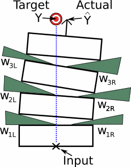
Recall that the goal is to adjust all the wedges until the actual value is where you want it. This value that the system actually produces for a given input is often marked as a Y with a hat on it. People even say "why-hat". Plain Y sans chapeau is used to designate what the target should be and thus what we are aiming for. In machine learning the plain Y is often the "label" part of a labeled training set. We want to adjust the system (weights) so that it at least hits these known targets pretty well before trying it on data we don’t have the correct answers for.
Looking over the diagram with the wedges, it’s almost simple enough now to actually do explicit geometric calculations. But I’m lazy so I need to simplify this yet more. We could imagine a big simplification by removing every other wedge and replacing it with a hinge.
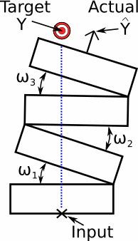
Now we’re down to just 3 knobs to adjust. I’ve made them omegas because that seems like a traditional angle sort of measurement and they still look like "w" which will remind us that these angle settings are now the "weights" in the system.
This is definitely doable, but I am even lazier than that. If we simplify this system even further we get something like this.
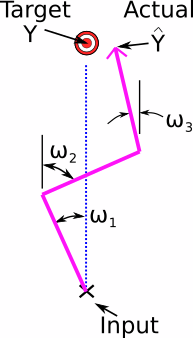
What’s cool about this format is that although it is structurally very similar to my previous conceptual model, it seems to have taken on a different form. This problem could be a robot arm with 3 servo motors. How would you set the servo motors to put the robot’s gripper on the target? In case you feel we’ve wandered too far away from machine learning, consider that this problem is just an optimization problem and so is machine learning. This highly stripped down version allows us to study it without tons of other complex considerations required by the scale of machine learning’s typical complexity. In other words, machine learning is basically solving problems like this; it’s just usually doing thousands at a time in parallel to be properly useful. We can just focus on one strand of the network that serendipitously has a different practical application.
This particular problem format is in fact an important problem on its own. It is called inverse kinematics and is critical to many fields from robotics to molecular physics. Now that I’ve evolved my tower of logs example into a simpler inverse kinematics problem, how can we solve it using the rough ideas also used at the heart of machine learning?
First let’s consider how we would figure out the structure’s current position given certain settings. If you recall very basic trigonometry and we assume that each segment of the linkage is one unit long, the positions of the joints are very easy to calculate. The lateral position is just the sine of that joint’s angle. We can keep an account of these as we go, each joint’s position added to the previous. Here is some simple code that takes a starting position where the base is located (Y0) and angle settings for each of three joints (w1,w2,w3), and returns the lateral position at each end point (Y1,Y2, and the end, Y3).
#!/usr/bin/python
from math import sin,cos,radians # This example involves trigonometry.

def calculate_pose(Y0,w1,w2,w3): # Base position and linkage angles.
    Y1= Y0 + sin(w1)             # First arm's end position.
    Y2= Y1 + sin(w2)             # Second arm's end position.
    Y3= Y2 + sin(w3)             # End of entire 3 bar linkage.
    return Y1,Y2,Y3              # Output lateral positions of linkage.
Pretty simple, right? This is the forward pass. We take the system and see how it is with no meddling. Seeing what you’ve got and how the system works out is the first step before messing with things to try and improve the system.
I’m trying to show a radically simplified example here so that the core ideas used in machine learning are less likely to be lost in the bustle of all of the other things necessary for useful deep learning neural networks in practice (a large network, more complex and less visual functions, a lot of data to apply statistics to, framework conventions, etc). So don’t fixate too much on the deficiencies. In most neural network lessons, you will start with a different kind of gross simplification. I feel having two different simple perspectives is helpful.
Once we know how well the system is working, i.e. how far Y3 is from being the same as Y0, we want to adjust the system (weights) so if we try again, we can hopefully do better. The huge difference between neural network techniques and the way humans usually solve these kinds of hard problems is that humans don’t explicitly calculate algorithmic guesses for how to adjust each of the weights. For a computer to attack such problems, this is exactly what must be done.
Since we have 3 weights (the joint angles) that can be adjusted which affect the desired goal, we need to figure out optimal amounts to tweak each of these angles. One might wonder why we can’t just solve for the final answer. In some simple cases maybe that’s possible, but even in this one there are many (infinite) settings of the weights that will line up the end of the arm with the base. Perhaps with more constraints you could just solve it but in practice the complexity will make that notion prohibitive. We just want to converge effectively on something that works with a simple algorithm because in neural networks we’ll be applying it a gazillion times.
The main gist of how this works is we consider in turn how each weight
affects the overall error. In other words, if I turn w1, how does the
Y3 end position change? Or similarly but more importantly how does the
distance to the target change? I’ll call that distance E for error
and unlike the position, Y3, it will always be positive. We ask
the same about w2 and w3. For people who can remember calculus, these
values are the derivatives of E (the error) with respect to each
weight. If I turn w1 quickly, does the error E change slowly or
quickly? Does it go up or down? That’s what we’re looking for.
Math people write
this quantity as a "dE" over "dw1" like a fraction (maybe even using
Greek deltas). As a programmer I’ll write it like dE_dw1.
The trick with machine learning often involves very elaborate networks of calculations that are as simple as I’ve contrived. It is generally necessary to calculate the change in error, dE, with respect to an intermediate thing changing and then calculate how that intermediate thing changes with respect to your important weight adjustment. There can be many layers of this. This is what back propagation really is.
With all that explained let’s continue with the program and see how we can figure out how to adjust the weights to lower the error.
def update_weights(Y0,w1,w2,w3):
    Y1,Y2,Y3= calculate_pose(Y0,w1,w2,w3)
Here’s a new function and the first thing to do is figure out where we’re at with the weights as they are. You could think of this first step as the forward pass or forward propagation.
    E= .5*(Y0-Y3)**2 # Magnitude of error.
    dE_dY3= -(Y0-Y3) # Change in error as Y3 changes (just Y3 for Y1=0).
This next bit looks ugly but is really not too bad. The E is the error
we want to minimize. We’re trying to make Y3 line up with the base at
Y0, so their differences need to be close to zero. The first line
just calculates the sum of the squared error,
SSE, to
prevent large negative errors from seeming better (smaller) than small
positive errors.
Next the derivative dE_dY3 is calculated. This is the change in error
E with respect to the change in Y3 (the position of the end of the
linkage). Obviously this is a very simplistic thing to worry about but
it is illustrative of the bulk of the work that is done in real neural
networks at deeper layers. This also shows why it’s often traditional
to multiply by 1/2 when calculating E (because the derivative of
.5*x*x simplifies to just x).
One thing I do remember from my many misspent years studying calculus is that the derivative of the sine function is, interestingly, the cosine function. This means that the rate of change in each arm’s position is related to the joint angle’s rate of change by cosine. That gives us this.
    dY3_dw1= cos(w1) # Rate of change of Y3 as w1 is adjusted.
    dY3_dw2= cos(w2) # Rate of change of Y3 as w2 is adjusted.
    dY3_dw3= cos(w3) # Rate of change of Y3 as w3 is adjusted.
But this isn’t exactly what we’re after. We need to link the adjustment of the joint with the final error and currently we have joint angle to position, and position to error. To chain these two steps together, we use a trick of calculus called the chain rule. When I learned the chain rule long ago, I was confident that it could be safely forgotten. But no! It’s actually quite useful and really at the heart of allowing neural network machine learning to be possible. If you want to brush up on your calculus, look carefully at the chain rule.
If getting your head around how exactly the chain rule works and why it is important seems hard, thankfully, just deploying it is refreshingly easy. Here it is in action.
    dE_dw1= dE_dY3 * dY3_dw1 # Chain rule.
    dE_dw2= dE_dY3 * dY3_dw2
    dE_dw3= dE_dY3 * dY3_dw3
Again, that’s a super simple example by design for educational purposes. In practice this will get ugly enough that you will definitely want a computer to keep track of things but conceptually, this is all there is to it.
After that step, we know how the error, E, is linked to each weight. Now comes the part where we actually adjust the weights. This introduces something called the "learning rate". Imagine I’m leveling my log tower by turning screws. I may feel like a full turn of screw J will bring down the error twice as much as a full turn of screw K. That’s super helpful (and basically what we have with dE_dw1, etc) but that still leaves an important practical question — how much should I actually turn those screws? I could turn K one turn and J two turns. Or I could turn K half a turn and J one turn. Or K 6 turns and J 12. We know which screws most effectively solve our problem relatively speaking but we don’t know how much of that solution to apply. The answer to this question is specified by the "learning rate". This is often shown with a greek letter eta (though other conventions are annoyingly common).
In neural network training, this is a hyperparameter which must be selected by the designer. You can imagine that 100 turns with K and 200 with J might overshoot your goals while 0.1 degree of J turning and 0.2 degrees of K might not accomplish enough to be useful in a reasonable amount of adjustment iterations. You just have to choose based on intuition and make revisions if it is not improving at a sensible pace.
Now the weights can be corrected using the original weights and the learning rate and the connection factor between the error and this weight. This is known as the delta rule though memorizing that fact doesn’t seem critical.
    eta= .075           # Learning rate. Chosen by trial and error.
    w1= w1 - eta*dE_dw1 # Delta rule.
    w2= w2 - eta*dE_dw2
    w3= w3 - eta*dE_dw3
    return w1,w2,w3     # New improved weights ready for another try!
And that is basically it. Now we just need to do this operation a decent number of times. Each time the metaphorical tower is disassembled, adjusted, and reassembled is called an "epoch".
Another surprisingly important technicality is choosing where the system starts from. This example is so simplified that if all the joints are set to zero, no further work is needed! But in real neural networks, the opposite is often true. By setting all the weights to zero initially, you often have a terrible time training it. It is common that performance is greatly enhanced with starting weights set randomly. Often subtle changes in this can have a huge impact on overall learning success. For example, maybe setting them with a Gaussian distribution versus just purely random noise. But in our little example, I’ll just pick some nice looking arbitrary starting angles.
Here then is the main program that actually iterates towards a solution.
Y0= 0                                          # Initial input.
w1,w2,w3= radians(22),radians(-20),radians(14) # Initial arbitrary weights.
print(calculate_pose(Y0,w1,w2,w3))             # Show initial pose.
for epoch in range(20):                        # Iterate through epochs.
    w1,w2,w3= update_weights(Y0,w1,w2,w3)      # Keep improving weights.
print(calculate_pose(Y0,w1,w2,w3))             # Show final pose.
When I run this I get the following output.
(0.374606593415912, 0.0325864500902433, 0.274508345689911)
(0.2852955778665301, -0.14244640527322044, 0.0029191436234602963)
These are the lateral displacements of the end of each arm segment. Since the overall objective was to get the end of my robot arm to line up with the base (which was zero), we were hoping that the final number would come down close to zero and it did!
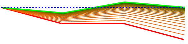
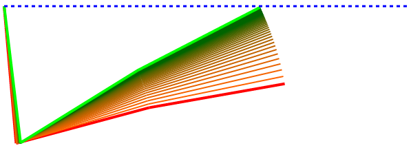
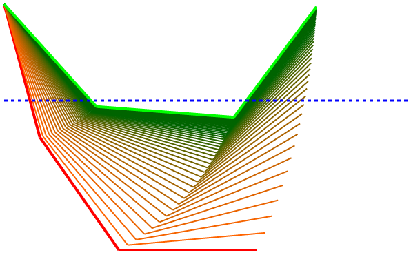
I ran this with a bunch more different starting weights so we can see how and how well the algorithm finds the desired solution. These diagrams show the starting pose as a red line and the final solution pose in green. This one shows an arm with the first joint at 10 degrees, the second set to 15, and the third set to 10 (these angles are all with respect to absolute horizontal, not the previous segment).
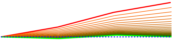
As you can see the initial pose quickly converges on the correct pose. The learning rate will influence how jumpy the transition is. The number of epochs controls how persistent it is and how many intermediate poses are attempted before returning a best guess final answer.
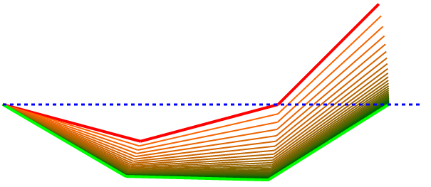
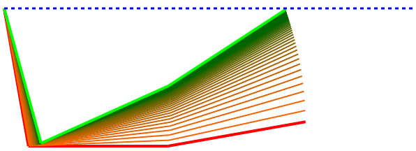
This one shows that even when the error is negative, this strategy still tries to minimize it back to a horizontal zero.
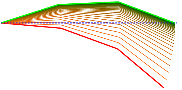
Here are some diverse examples showing that it can pretty reliably and sensibly find a solution.
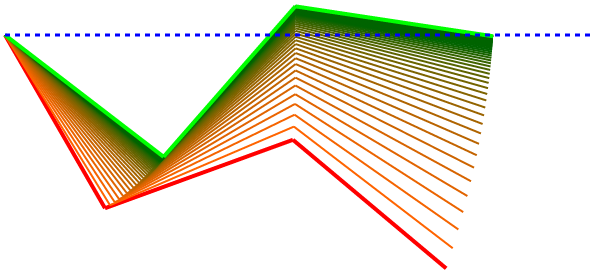
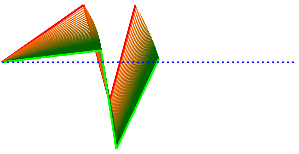
These next two show that the algorithm isn’t perfect. By prioritizing adjustments based on the derivatives, you can see that this cosine strategy penalizes valid improvements where the angles are close to 90. When the angle is close to 90, the cosine (derivative of the position’s function, sine) is close to zero so not much gets improved at that location even though it could theoretically be doing more to help.
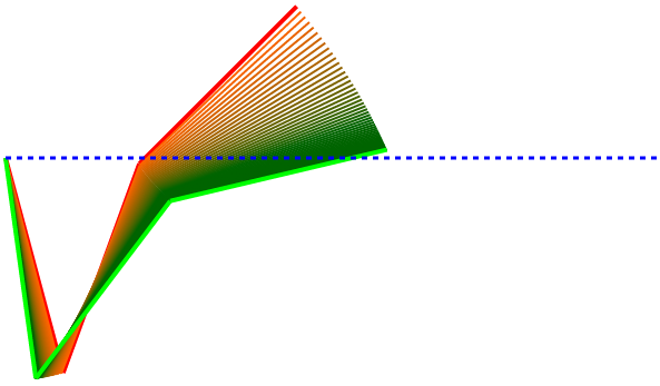
This one seems even worse even if it did manage to find a solution.
This next one did struggle to find a satisfactory solution in the number of epochs I allowed.
For this next one, I changed the Y0 value to be 0.7 which merely shifts the whole thing up.
We could easily set up this system so that the target (Y3) and the input (Y0) could be different and this would allow us to move a robot arm to arbitrary elevations. Traditionally the input to the system (not the weights which are the system) is called X but in a graphical geometric example, that is a bit confusing.
The big leap from this simple example to proper machine learning are systems where the input vector X (Y0 here) can be novel previously unseen circumstances and, because the weights are set (trained) so cleverly, the output reflects some useful insight. For example, you could imagine putting the input (Y0) at the number of legs a creature has and training the system with a lot of examples until the system’s weights can position the end of the arm below zero for mammals and above zero for insects. We know from general experience that the math is pretty simple there (4 or less legs, probably not an insect) but that is something the system can start to figure out on its own if you keep giving it known examples (number of legs and correct invertebrate status). The functions of how the joint angles are set by the weights (purely geometric and in the simplest way possible in my example) may need to be upgraded to allow more complexity and quirky outcomes but that’s exactly what you’ll find in proper neural network architectures.
Machine learning involves going through lots of examples just like this one and finding the best ways to adjust the weights so that the entire collection of these training examples produce results as close to what you want as possible. Then, and this is the entire point, you can give it a new input and its best guess about it will hopefully be pretty useful.